Shaping electric power system with historical weather
Overview
The set of USENSYS scenarios in this mini-study takes historical hourly weather data to evaluate the potential of intermittent renewables and optimize electric power system structure from scratch, disregarding the existing generating capacity and the existing power network. The exercise sketches the potential structure of the US electric power sector if entirely based on renewables; evaluates the role of energy storage and long-distance power grid in high-renewables power system; estimates reliability, curtailments, and average system costs of electricity generation.
Purpose
Brainstorming/sketching the potential structure of US electric power system if entirely based on intermittent renewables, using historical weather data (MERRA-2 project by NASA), generic technologies (wind turbines, solar PVs, energy storage, ultra-high voltage power grid) with realistic costs and electricity consumption, asking the questions:
- How the US electric power system would look like if built from scratch 100% based on renewable energy?
- Is it technically feasible to rely solely on solar or/and wind energy for electricity generation, balancing it with energy storage and long-distance grid to satisfy hourly electric demand by states (equivalent to 2018)?
- What would be the expected levelized systemwide costs of electricity of a 100%-renewables power system?
- What would be the cost-optimal capacity structure of solar- and wind-power generation?
- How availability and costs of energy storage, long-distance grid, solar and wind power technologies would affect the cost-optimal structure of the power system?
Every particular scenario is not nessasarily practical or suggested for application. Rather it markes the line of technical feasibility and the magnitude of costs of such state of the system. The results might contribute to a broader discussion of a technical feasibility and economic rationale of a high-renewables electric power system in the US, as well as help to identify directions for further research.
Main assumptions and simplifications
(see USA_ELC_BAL_R49_v04.Rmd for detailed specification of the model.)
Regions:
- 48 lower states and DC.
Time resolution: - 1 year, 8760 hours (24 hours * 365 days).
Technologies: - Solar photovoltaics (PVs, $1/Watt, 1sq.m PV requires ~2.5sq.m of land - not met);
- Onshore wind turbines ($1.5/Watt, land use ~3 MW/km2 );
- Offshore wind turbines ($3.5/Watt, land use ~5 MW/km2);
- Generic energy storage ($300 USD/kWh, 80% efficiency);
- Long distance (UHVDC) power lines ($200 MUSD/GW for 1000 km of 1GW line + 50% costs of land).
The resource of renewables: - Estimated based on MERRA-2 data (see the model details).
- the potential output of solar PVs is estimated based on solar direct radiation flux for every hour and the grid cell (around 30 by 60 miles for US latitude) of MERRA-2 data.
- the potential output of wind turbines is estimated based on the average wind speed for every hour and the grid cell, using a wind power output curve. The locations with the best potential output over the year are selected for every state.
- The potential output of renewables in every region is calculated as an average output from the potential solar or wind-power, assuming the uniform distribution of the capacities across the selected territories. [The estimate of the resource potential might be improved by narrowing down locations available for installation, as well as using more granular data and will be considered on further steps.]
Land: - Costs of the land, required for solar PVs and wind turbines are not considered on this stage, making the main focus on the physical resource. The costs of land for UHVDC are assumed to be included in the investment costs of the technology.
Demand: - Hourly demand by states, estimated based on monthly power generation by states and national hourly power load curve.
Reliability: - the cut-off costs of marginal electricity is $10 USD/kWh, i.e. the model will not invest in any capacity to deliver electricity with marginal costs higher than the cut-off in a particular hour; the unsatisfied demand is reported as “demand curtailments”.
On uncertainty: - While a weather-driven power generation incorporates some uncertainty by default, there is no uncertainty in the optimization routine. The cost-minimizing linear programming problem is solved under an assumption of the full information. I.e. the system is shaped based on minimal costs, taking into account historical weather, hourly demand, costs and parameters of thechnologies; the potential output in a particular hour and region is known, as well as the demand. Therefore the system is optimzed for this particular state of the input parameters. Changing the historical weather year will affect the optimal (for a given year) structure of the system. Robustness tests for each particular shape of the system subject to different years of the weather will be considered on further steps.
Scenarios
The following scenarios optimize electric power system based on solar- and/or wind- generation (individually or combined) with different assumptions regarding availability of the generating technologies and interregional UHVDC grid.
1. “Sunny home”
A hypothetical scenario for 2018 where every state generates electricity with solar PVs, no inter-regional dispatch. The scenario evaluates the required capacity of PVs and the storage to meet hourly electric demand, estimates supply curtailments, the power system failiture to satisfy the demand, and the total system costs.
The scenario-specific assumptions:
- Solar PVs are the only generating technologies;
- No interregional dispatch (the local interstate grid is assumed but not modeled in all scenarios);
- Generic storage (alike batteries, distributed or local-grid-connected).
code
repo_sun <- add(newRepository('main_repository'),
  # Commodities
  ELC, SOL, # WIN, WFF, #UHV,
  # Resources (supply)
  RES_SOL, # RES_WIN, RES_WFF,
  # Weather factors
  SOLAR_AF, # WINOF20_AF, WINON20_AF,
  CSOL_UP, # CWIN_UP, CWFF_UP,
  # Generating technologies
  ESOL, # EWIN, EWFF,
  # Storage
  STGBTR,
  # UHV grid
  # TRBD_UHV_NEI,
  # ELC2UHV, UHV2ELC,
  # Export/Import (curtailments),
  # EEXP,
  EIMP,
  # ELC demand with load curve (24 hours x 365 days)
  DEM_ELC_DH # static
)
length(repo_sun@data)
names(repo_sun@data)

mod <- newModel(
  name = 'SUNNY',
  description = "Sunny home scenario",
  region = reg_names,
  discount = 0.05,
  slice = list(ANNUAL = "ANNUAL",
               YDAY = timeslices365$YDAY,
               HOUR = timeslices365$HOUR
               ),
  repository = repo_sun,
  GIS = usa49reg,
  early.retirement = F)

# Check the model time-slices
head(mod@sysInfo@slice@levels)

# Set milestone-years
mod <- setMilestoneYears(mod, start = 2018, interval = c(1))
mod@sysInfo@milestone # check

# (optional) GAMS and CPLEX options
# mod@misc$includeBeforeSolve <- cplex_options
# mod@misc$includeBeforeSolve <- GAMS$inc3
# # (optional) save GDX file with the solution
# mod@misc$includeAfterSolve <- inc_after_solve
{mod@description <- "
USENSYS, power sector, renewables balancing version,
49 regions, 1 hour resolution,
1 types of renewables (solar PVs),
1 types of storages,
no interregional dispatch (grid),
no initial capacity stock."}

# 1. Interpolation of parameters
scen_SUNNYHOME <- interpolate(mod, name = "SUNNYHOME",
  description = "No inter-regional dispatch.")
size(scen_SUNNYHOME)

# 2. Writing the model's code with the data on disk
write_model(scen_SUNNYHOME, tmp.dir = "solwork/scen_SUNNYHOME", solver = GAMS)
# write_model(scen_SUNNYHOME, tmp.dir = "solwork/scen_SUNNYHOME_py", solver = PYOMO)
# JuMP = list(lang = "JuMP", solver = "CPLEX")
# write_model(scen_SUNNYHOME, tmp.dir = "solwork/scen_SUNNYHOME_jl", solver = JuMP)
# save(scen_SUNNYHOME, file = "solwork/scen_SUNNYHOME.RData")

# 3. Solving the model
solve_model("solwork/scen_SUNNYHOME", wait = FALSE)
# solve_model("solwork/scen_SUNNYHOME_py", wait = FALSE, invisible = FALSE)
# solve_model("solwork/scen_SUNNYHOME_jl7", wait = FALSE)


# 4. Read the solution (run manually once the model is solved)
if (F) {
  scen_SUNNYHOME <- read_solution(scen_SUNNYHOME, dir.result = "solwork/scen_SUNNYHOME")
  # scen_SUNNYHOME_py <- read_solution(scen_SUNNYHOME, dir.result = "solwork/scen_SUNNYHOME_py")
  summary(scen_SUNNYHOME)
  # summary(scen_SUNNYHOME_py)

  # ll <- lcompare(scen_SUNNYHOME_gms@modInp, scen_SUNNYHOME_py@modInp)
  # ll <- lcompare(scen_SUNNYHOME_gms@modInp@set, scen_SUNNYHOME_py@modInp@set)
  # ll <- lcompare(scen_SUNNYHOME_gms@modOut, scen_SUNNYHOME_py@modOut)
  # size(ll)
  # names(ll)
  # size(ll$sets, 1)
  # ll$sets$region

  save(scen_SUNNYHOME, file = "scenarios/scen_SUNNYHOME.RData")
}
2. “Sunny Arizona”
The scenario restricts installation of PVs to one state - Arizona with a goal to evaluate the impact on electricity costs and UHVDC network.
The scenario-specific assumptions:
- Solar PVs are the only generating technologies;
- Arizona is the only state which can produce electricity (from solar PVs);
- Endogenous interregional dispatch (100 UHVDC lines between neighbor regions);
- Storage (alike batteries, distributed or local-grid-connected).
code
ESOL_AZ <- ESOL
ESOL_AZ@region <- "AZ" # limiting the technology to one region
CSOL_UP_AZ <- newConstraintS(
  name = "CSOL_UP",
  eq = "<=",
  type = "capacity",
  for.each = data.frame(
    year = USENSYS$modelYear,
    tech = "ESOL",
    region = "AZ"),
  rhs = PV_GW_max_reg$GW_up[PV_GW_max_reg$region == "AZ"] * 5 # relaxing the constraint
  ) # limit on solar capacity (resource)


# 1. Interpolation of parameters
scen_SUNNYAZ <- interpolate(
  add(mod, ESOL_AZ, CSOL_UP_AZ, TRBD_UHV_NEI, UHV, ELC2UHV, UHV2ELC, overwrite = T),
  name = "SUNNYAZ", #n.threads = 4,
  description = "Arizona is the only state to generate electricity (from solar energy).")
summary(scen_SUNNYAZ)
size(scen_SUNNYAZ)
# save(scen_SUNNYAZ, file = "tmp/scen_SUNNYAZ_interpolated.RData")

# 2. Writing the model's code with the data on disk
write_model(scen_SUNNYAZ, tmp.dir = "solwork/scen_SUNNYAZ", solver = GAMS)
# write_model(scen_SUNNYAZ, tmp.dir = "solwork/scen_SUNNYAZ_pkgv04", solver = "GAMS")
# solve_model(tmp.dir = "solwork/scen_SUNNYAZ_pkgv04", wait = FALSE)
# scen_SUNNYAZ <- read_solution(scen_SUNNYAZ, dir.result = "solwork/scen_SUNNYAZ_pkgv04")
# summary(scen_SUNNYAZ)
# save(scen_SUNNYAZ, file = "solwork/scen_SUNNYAZ_pkgv04.RData")
# write_model(scen_SUNNYAZ, tmp.dir = "solwork/scen_SUNNYAZ_jl", solver = JuMP)
# solve_model("solwork/scen_SUNNYAZ_jl", wait = FALSE)

# 3. Solving the model
solve_model("solwork/scen_SUNNYAZ", wait = FALSE)

# 4. Read the solution (run manually once the model is solved)
if (F) {
  scen_SUNNYAZ <- read_solution(scen_SUNNYAZ, dir.result = "solwork/scen_SUNNYAZ")
  summary(scen_SUNNYAZ)

  save(scen_SUNNYAZ, file = "scenarios/scen_SUNNYAZ.RData")
}
3. “Sharing the Sun”
Adding UHVDC grid as an investment option to the scenario #1. There is no upper limit on any investments. The capacity structure including the power network is shaped based on minimal overal system costs.
code
# 1. Interpolation of parameters
scen_SUNSHARE <- interpolate(
  add(mod, TRBD_UHV_NEI, UHV, ELC2UHV, UHV2ELC),
  name = "SUNSHARE",
  description = "Solar energy and interregional dispatch.")
size(scen_SUNSHARE)

# 2. Writing the model's code with the data on disk
write_model(scen_SUNSHARE, tmp.dir = "solwork/scen_SUNSHARE", solver = GAMS)
# save(scen_SUNSHARE, file = "solwork/scen_SUNSHARE.RData")

# write_model(scen_SUNSHARE, tmp.dir = "solwork/scen_SUNSHARE_jl", solver = JuMP)
# solve_model("solwork/scen_SUNSHARE_jl", wait = FALSE)

# 3. Solving the model
solve_model("solwork/scen_SUNSHARE", wait = FALSE)

# 4. Read the solution (run manually once the model is solved)
if (F) {
  scen_SUNSHARE <- read_solution(scen_SUNSHARE, dir.result = "solwork/scen_SUNSHARE")
  summary(scen_SUNSHARE)

  save(scen_SUNSHARE, file = "scenarios/scen_SUNSHARE.RData")
}
4. “Sharing the Sun 50”
The scenario sets limits on investments in UHVDC network, 50% upper bound of the resulting UHVDC investments in Scenario #3. Investments in particular UHVDC lines are not limited.
code
# Grid constraints % of SUNSHARE.
if (exists("scen_SUNSHARE")) {
  # Unrestricted (optimal) grid capacity from SUNSHARE
  # load("scenarios/scen_SUNSHARE.RData")
  msy <- mod@sysInfo@milestone$mid

  (vTradeCap <- getData(scen_SUNSHARE, name = "vTradeCap", merge = T, year = max(msy),
                        newNames = c(value = "GW")))

  trd_TWkm <- full_join(trd_dt, select(vTradeCap, trade, GW)) %>%
    mutate(TWkm = distance_km / 1e3 * GW)
  sum(trd_TWkm$TWkm, na.rm = T) # TW*km

  # Unrestricted (optimal) grid investment in SUNSHARE
  (vTradeInv <- getData(scen_SUNSHARE, name = "vTradeInv", merge = T))
  sum(vTradeInv$value) # MRMB
  sum(vTradeInv$value)/sum(trd_TWkm$TWkm, na.rm = T)

  GRIDINV50_SUNSHARE <- newConstraint(
    'GRIDINV50_SUNSHARE', eq = '<=', rhs = sum(vTradeInv$value)/2,
    variable = list(variable = 'vTradeInv'))

  GRIDINV25_SUNSHARE <- newConstraint(
    'GRIDINV25_SUNSHARE', eq = '<=', rhs = sum(vTradeInv$value)/4,
    variable = list(variable = 'vTradeInv'))

  GRIDINV10_SUNSHARE <- newConstraint(
    'GRIDINV10_SUNSHARE', eq = '<=', rhs = sum(vTradeInv$value)/10,
    variable = list(variable = 'vTradeInv'))

  GRIDINV05_SUNSHARE <- newConstraint(
    'GRIDINV05_SUNSHARE', eq = '<=', rhs = sum(vTradeInv$value)/20,
    variable = list(variable = 'vTradeInv'))

  GRIDINV01_SUNSHARE <- newConstraint(
    'GRIDINV01_SUNSHARE', eq = '<=', rhs = sum(vTradeInv$value)/100,
    variable = list(variable = 'vTradeInv'))


} # Grid constraints % of SUNSHARE
# 1. Interpolation of parameters
scen_SUNSHARE50 <- interpolate(
  add(mod, TRBD_UHV_NEI, UHV, ELC2UHV, UHV2ELC, GRIDINV50_SUNSHARE),
  name = "SUNSHARE50",
  description = "Solar energy and interregional dispatch with 50% constraint on investment.")
size(scen_SUNSHARE50)

# 2. Writing the model's code with the data on disk
write_model(scen_SUNSHARE50, tmp.dir = "solwork/scen_SUNSHARE50", solver = GAMS)
# save(scen_SUNSHARE50, file = "solwork/scen_SUNSHARE50.RData")

# 3. Solving the model
solve_model("solwork/scen_SUNSHARE50", wait = FALSE)

# 4. Read the solution
if (F) {
  scen_SUNSHARE50 <- read_solution(scen_SUNSHARE50, dir.result = "solwork/scen_SUNSHARE50")
  summary(scen_SUNSHARE50)

  save(scen_SUNSHARE50, file = "scenarios/scen_SUNSHARE50.RData")
}
5. “Windy states”
The scenario similar to the #3 “Sharing the Sun”, with the difference that the wind power is used instead of solar.
code
# Reformulate the model for the wind energy
repo_wnd <- add(newRepository('main_repository'),
            # Commodities
            ELC, UHV,
            SOL,
            WIN, WFF,
            # Resources (supply)
            # RES_SOL,
            RES_WIN, RES_WFF,
            # CSOL_UP,
            CWIN_UP, CWFF_UP,
            # Weather factors
            # SOLAR_AF,
            WINOF20_AF, WINON20_AF,
            # Generating technologies
            # ESOL,
            EWIN, EWFF,
            # Storage
            STGBTR,
            # STGBTR1, #STGP2P1,
            # Simplified interregional ELC trade
            # UHV grid
            TRBD_UHV_NEI,
            ELC2UHV, UHV2ELC,
            # Export/Import,
            EEXP, EIMP,
            # ELC demand with load curve (24 hours x 365 days)
            DEM_ELC_DH # static
)
length(repo_wnd@data)
names(repo_wnd@data)

mod_wnd <- newModel(
  name = 'WINDY',
  description = "Wind only",
  region = reg_names,
  discount = 0.05,
  slice = list(ANNUAL = "ANNUAL",
               YDAY = timeslices365$YDAY,
               HOUR = timeslices365$HOUR
  ),
  repository = repo_wnd,
  GIS = usa49reg,
  early.retirement = F)

# Check the model time-slices
head(mod_wnd@sysInfo@slice@levels)

# Set milestone-years
mod_wnd <- setMilestoneYears(mod_wnd, start = 2018, interval = c(1))
mod_wnd@sysInfo@milestone # check

{mod_wnd@description <- "
USENSYS, power sector, renewables balancing version,
49 regions, 1 hour resolution,
1 types of renewables (Wund turbines),
1 types of energy storages,
UHVDC interregional dispatch as an investment option,
no initial capacity stock."}

# (optional) GAMS and CPLEX options
mod_wnd@misc$includeBeforeSolve <- cplex_options
# (optional) save GDX file with the solution
mod_wnd@misc$includeAfterSolve <- inc_after_solve

scen_WINDY <- interpolate(
  mod_wnd,
  name = "WINDY",
  description = "Windy states: Wind energy, UHVDC grid, and storage.")
size(scen_WINDY)

# 2. Writing the model's code with the data on disk
write_model(scen_WINDY, tmp.dir = "solwork/scen_WINDY", solver = GAMS)
# save(scen_WINDY, file = "solwork/scen_WINDY.RData")

# 3. Solving the model
solve_model("solwork/scen_WINDY", wait = FALSE)

# 4. Read the solution
if (F) {
  scen_WINDY <- read_solution(scen_WINDY, dir.result = "solwork/scen_WINDY")
  summary(scen_WINDY)

  save(scen_WINDY, file = "scenarios/scen_WINDY.RData")
}
6. “The Wind and the Sun”
Both intermittent energy sources - wind and solar can be used to generate electricity. The scenario is similar to the combined #3 and #5 (wind or solar work togeather).
code
# reformulate the model
repo_ren <- add(newRepository('main_repository'),
                # Commodities
                ELC, UHV,
                SOL,
                WIN, WFF,
                # Resources (supply)
                RES_SOL, RES_WIN, RES_WFF,
                CSOL_UP, CWIN_UP, CWFF_UP,
                # Weather factors
                SOLAR_AF,
                WINOF20_AF, WINON20_AF,
                # Generating technologies
                ESOL,
                EWIN, EWFF,
                # Storage
                STGBTR,
                # STGBTR1, #STGP2P1,
                # Simplified interregional ELC trade
                # UHV grid
                TRBD_UHV_NEI,
                ELC2UHV, UHV2ELC,
                # Export/Import,
                # EEXP,
                EIMP,
                # ELC demand with load curve (24 hours x 365 days)
                DEM_ELC_DH # static
)
length(repo_ren@data)
names(repo_ren@data)

mod_ren <- newModel(
  name = 'WINSUN',
  description = "Wind only",
  region = reg_names,
  discount = 0.05,
  slice = list(ANNUAL = "ANNUAL",
               YDAY = timeslices365$YDAY,
               HOUR = timeslices365$HOUR
  ),
  repository = repo_ren,
  GIS = usa49reg,
  early.retirement = F)

# Check the model time-slices
head(mod_ren@sysInfo@slice@levels)

# Set milestone-years
mod_ren <- setMilestoneYears(mod_ren, start = 2018, interval = c(1))
mod_ren@sysInfo@milestone # check

{mod_ren@description <- "
USENSYS, power sector, renewables balancing version,
49 regions, 1 hour resolution,
2 types of renewables (solar PVs, wind turbines),
1 types of storages,
UHVDC interregional dispatch as an investment option,
no initial capacity stock."}

# (optional) GAMS and CPLEX options
# mod_ren@misc$includeBeforeSolve <- cplex_options
# (optional) save GDX file with the solution
# mod_ren@misc$includeAfterSolve <- inc_after_solve

scen_WINSUN <- interpolate(
  add(mod_ren),
  name = "WINSUN",
  description = "Wind & solar energy, UHVDC grid")
size(scen_WINSUN)
summary(scen_WINSUN)

# 2. Writing the model's code with the data on disk
write_model(scen_WINSUN, tmp.dir = "solwork/scen_WINSUN", solver = GAMS)
# write_model(scen_WINSUN, tmp.dir = "solwork/scen_WINSUN_py", solver = "PYOMO")
save(scen_WINSUN, file = "solwork/scen_WINSUN.RData")

# 3. Solving the model
solve_model("solwork/scen_WINSUN", wait = FALSE)

# 4. Read the solution
if (F) {
  scen_WINSUN <- read_solution(scen_WINSUN, dir.result = "solwork/scen_WINSUN")
  summary(scen_WINSUN)

  save(scen_WINSUN, file = "scenarios/scen_WINSUN.RData")
}
7. “The Wind and the Sun 50”
Similar to #6 with an added limit on investment in UHVDC power lines, 50% of unrestricted cost-optimal (scenario #6).
code
# Grid constraints % of WINSUN
if (exists("scen_WINSUN")) {
  # Unrestricted (optimal) grid capacity from WINSUN
  # load("scenarios/scen_WINSUN.RData")
  msy <- mod_ren@sysInfo@milestone$mid

  (vTradeCap <- getData(scen_WINSUN, name = "vTradeCap", merge = T, year = max(msy),
                        newNames = c(value = "GW")))

  trd_TWkm <- full_join(trd_dt, select(vTradeCap, trade, GW)) %>%
    mutate(TWkm = distance_km / 1e3 * GW)
  sum(trd_TWkm$TWkm, na.rm = T) # TW*km

  # Unrestricted (optimal) grid investment in WINSUN
  (vTradeInv <- getData(scen_WINSUN, name = "vTradeInv", merge = T))
  sum(vTradeInv$value) # MRMB
  sum(vTradeInv$value)/sum(trd_TWkm$TWkm, na.rm = T)

  GRIDINV50_WINSUN <- newConstraint(
    'GRIDINV50_WINSUN', eq = '<=', rhs = round(sum(vTradeInv$value)/2, -2),
    variable = list(variable = 'vTradeInv'))

  GRIDINV25_WINSUN <- newConstraint(
    'GRIDINV25_WINSUN', eq = '<=', rhs = sum(vTradeInv$value)/4,
    variable = list(variable = 'vTradeInv'))

  GRIDINV10_WINSUN <- newConstraint(
    'GRIDINV10_WINSUN', eq = '<=', rhs = sum(vTradeInv$value)/10,
    variable = list(variable = 'vTradeInv'))

  GRIDINV05_WINSUN <- newConstraint(
    'GRIDINV05_WINSUN', eq = '<=', rhs = sum(vTradeInv$value)/20,
    variable = list(variable = 'vTradeInv'))

  GRIDINV01_WINSUN <- newConstraint(
    'GRIDINV01_WINSUN', eq = '<=', rhs = sum(vTradeInv$value)/100,
    variable = list(variable = 'vTradeInv'))


} # Grid constraints % of WINSUN
scen_WINSUN50 <- interpolate(
  add(mod_ren, GRIDINV50_WINSUN),
  name = "WINSUN50",
  description = "Wind & solar energy, UHVDC grid 50% limit")
size(scen_WINSUN50)

# 2. Writing the model's code with the data on disk
write_model(scen_WINSUN50, tmp.dir = "solwork/scen_WINSUN50", solver = GAMS)
# save(scen_WINSUN50, file = "solwork/scen_WINSUN50.RData")

# 3. Solving the model
solve_model("solwork/scen_WINSUN50", wait = FALSE)

# 4. Read the solution
if (F) {
  scen_WINSUN50 <- read_solution(scen_WINSUN50, dir.result = "solwork/scen_WINSUN50")
  summary(scen_WINSUN50)

  save(scen_WINSUN50, file = "scenarios/scen_WINSUN50.RData")
}
8. “The Wind and the Sun 25”
Similar to #6 with added limit on investment in UHVDC power lines, 25% of unrestricted cost-optimal (scenario #6).
code
scen_WINSUN25 <- interpolate(
  add(mod_ren, GRIDINV25_WINSUN),
  name = "WINSUN25",
  description = "Wind & solar energy, UHVDC grid 25% limit")
size(scen_WINSUN25)

# 2. Writing the model's code with the data on disk
write_model(scen_WINSUN25, tmp.dir = "solwork/scen_WINSUN25", solver = GAMS)
# save(scen_WINSUN25, file = "solwork/scen_WINSUN25.RData")

# 3. Solving the model
solve_model("solwork/scen_WINSUN25", wait = FALSE)

# 4. Read the solution
if (F) {
  scen_WINSUN25 <- read_solution(scen_WINSUN25, dir.result = "solwork/scen_WINSUN25")
  summary(scen_WINSUN25)

  save(scen_WINSUN25, file = "scenarios/scen_WINSUN25.RData")
}
Comparative figures and tables
code
if (!exists("scen_SUNNYHOME")) load(file.path(homedir, "scenarios/scen_SUNNYHOME.RData"))
if (!exists("scen_SUNNYAZ")) load(file.path(homedir, "scenarios/scen_SUNNYAZ.RData"))
if (!exists("scen_SUNSHARE")) load(file.path(homedir, "scenarios/scen_SUNSHARE.RData"))
if (!exists("scen_SUNSHARE50")) load(file.path(homedir, "scenarios/scen_SUNSHARE50.RData"))
if (!exists("scen_WINDY")) load(file.path(homedir, "scenarios/scen_WINDY.RData"))
if (!exists("scen_WINSUN")) load(file.path(homedir, "scenarios/scen_WINSUN.RData"))
if (!exists("scen_WINSUN50")) load(file.path(homedir, "scenarios/scen_WINSUN50.RData"))
if (!exists("scen_WINSUN25")) load(file.path(homedir, "scenarios/scen_WINSUN25.RData"))

sns <- list(
  "1. Sunny Home" = scen_SUNNYHOME,
  "2. Sunny Arizona" = scen_SUNNYAZ,
  "3. Sharing the Sun" = scen_SUNSHARE,
  "4. Sharing the Sun 50" = scen_SUNSHARE50,
  "5. Windy States"  = scen_WINDY,
  "6. The Wind and the Sun" = scen_WINSUN,
  "7. The Wind and the Sun 50" = scen_WINSUN50,
  "8. The Wind and the Sun 25" = scen_WINSUN25
)

# Functions
add_centers <- function(df, centers = reg_centers[,1:3]) {
  # browser()
  if (any(names(df) == "trade") & !any(c("src", "dst") %in% names(df))) {
    df$src <- substr(df$trade, nchar(df$trade)-4, nchar(df$trade)-3)
    df$dst <- substr(df$trade, nchar(df$trade)-1, nchar(df$trade)-0)
  }

  if (all(c("src", "dst") %in% names(df))) {
    df <- df %>%
      left_join(centers, by = c("src" = "region")) %>%
      left_join(centers, by = c("dst" = "region")) %>%
      rename(x.src = x.x, y.src = y.x,
             x.dst = x.y, y.dst = y.y)
    df
  } else if ("region" %in% names(df)) {
    df %>%
      left_join(centers, by = c("region"))
    df
  } else {
    stop("`region` or `src` & `dst` columns have not been found")
  }
}
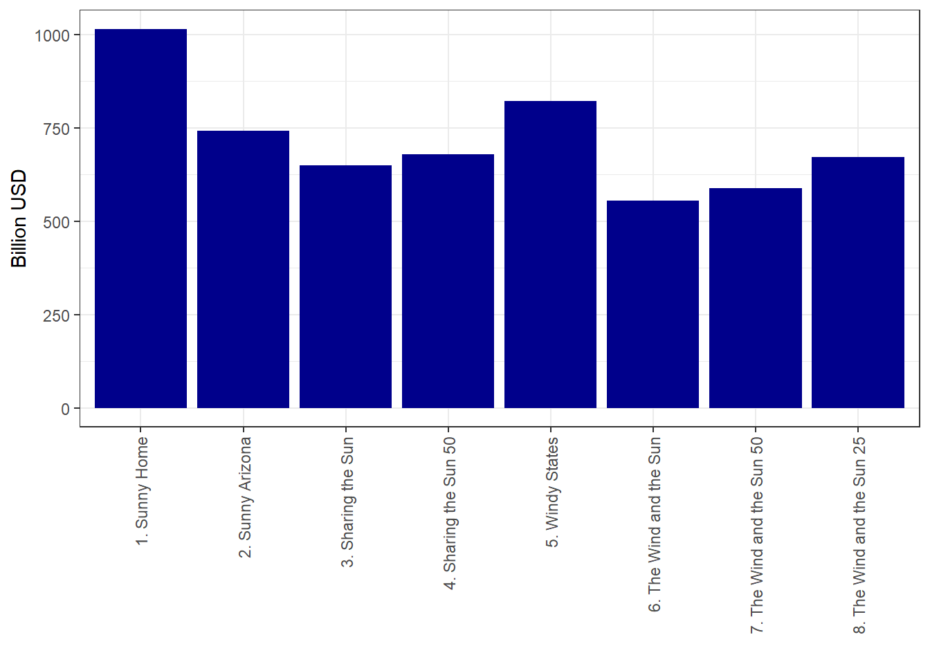
Annualized system costs (objective)
code
# Objective
vObjective <- getData(sns, name = "vObjective", merge = T) %>%
  group_by(scenario) %>%
  summarise(`Billion USD` = round(sum(value)/1e3, 2))

## Penalty for undelivered electricity
vImportCost <- getData(sns, c("vImportRow"), merge = T)
if (!is.null(vImportCost)) {
  pImportRowPrice <- EIMP@imp$price[1] # one import commodity,
  vImportCost <- vImportCost %>%
    group_by(scenario) %>%
    summarise(GWh = sum(value, na.rm = TRUE)) %>%
    mutate(ImpCost = pImportRowPrice * GWh)
  vObjective <- full_join(vObjective, vImportCost, by = "scenario") %>%
    mutate(`Billion USD` = `Billion USD` - round(if_else(is.na(ImpCost), 0, ImpCost)/1e3, 2)) %>%
    select(scenario, `Billion USD`)
}

# Credit for excess electricity
# vExportCost <- getData(sns, c("vExportRow"), merge = T)
# if (!is.null(vExportCost)) {
#   pExportRowPrice <- EEXP@exp$price[1]
#   vExportCost <- vExportCost %>%
#   group_by(scenario) %>%
#   summarise(GWh = sum(value, na.rm = TRUE)) %>%
#   mutate(ExpCost = pExportRowPrice * GWh)
#   vObjective <- full_join(vObjective, vExportCost, by = "scenario", na_matches = 0) %>%
#     mutate(`Billion USD` = `Billion USD` + round(if_else(is.na(ExpCost), 0, ImpCost)/1e3, 2)) %>%
#     select(scenario, `Billion USD`)
# }

tbl <- kable(vObjective) %>%
  kable_styling(bootstrap_options = c("striped", "hover", "condensed", "responsive"), full_width = T, position = "center")

plt <- ggplot(vObjective) +
  geom_bar(aes_string(x = "scenario", y = "`Billion USD`"),
           stat = "identity", fill = "darkblue") +
  theme_bw() +
  theme(axis.text.x = element_text(angle = 90, hjust = 1, vjust = .5)) +
  xlab("")
| scenario | Billion USD |
|---|---|
| 1. Sunny Home | 1014.95 |
| 2. Sunny Arizona | 742.13 |
| 3. Sharing the Sun | 649.27 |
| 4. Sharing the Sun 50 | 679.03 |
| 5. Windy States | 821.35 |
| 6. The Wind and the Sun | 555.20 |
| 7. The Wind and the Sun 50 | 587.83 |
| 8. The Wind and the Sun 25 | 671.73 |
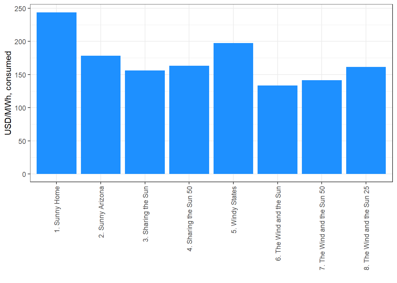
Average systemwide costs of electricity at consumer
code
pDemand <- getData(sns, "pDemand", merge = T) %>%
  group_by(scenario) %>%
  summarise("Demand, GWh" = sum(value))

vGen <- getData(sns, "vTechOut", comm = "ELC", tech_ = "^E", merge = T) %>%
  group_by(scenario) %>%
  summarise("Generation, GWh" = round(sum(value), 2))

vImportRow_ELC <- getData(sns, "vImportRow", comm = "ELC", merge = T) %>%
  group_by(scenario) %>%
  summarise("Demand curtailments, GWh" = sum(value))


elccost <-
  full_join(vObjective, pDemand, by = "scenario") %>%
  full_join(vGen, by = "scenario") %>%
  full_join(vImportRow_ELC, by = "scenario") %>%
  mutate(
    `Supply curtailments, %` = round(`Generation, GWh` / `Demand, GWh` * 100 - 100, 2),
    `Demand curtailments, %` = round(`Demand curtailments, GWh` / `Demand, GWh` * 100, 2),
    `USD/MWh, produced` = round(convert("MUSD/GWh", "USD/MWh", `Billion USD` / `Generation, GWh` * 1e3), 2),
    `USD/MWh, consumed` = round(convert("MUSD/GWh", "USD/MWh", `Billion USD` / `Demand, GWh` * 1e3), 2)
    )

tbl <- kable(elccost[,-5]) %>%
  kable_styling(bootstrap_options = c("striped", "hover", "condensed", "responsive"))
                # full_width = F, position = "center")
| scenario | Billion USD | Demand, GWh | Generation, GWh | Supply curtailments, % | Demand curtailments, % | USD/MWh, produced | USD/MWh, consumed |
|---|---|---|---|---|---|---|---|
| 1. Sunny Home | 1014.95 | 4161304 | 15065110 | 262.03 | 0.31 | 67.37 | 243.90 |
| 2. Sunny Arizona | 742.13 | 4161304 | 12217908 | 193.61 | 0.18 | 60.74 | 178.34 |
| 3. Sharing the Sun | 649.27 | 4161304 | 10142656 | 143.74 | 0.02 | 64.01 | 156.03 |
| 4. Sharing the Sun 50 | 679.03 | 4161304 | 10634609 | 155.56 | 0.12 | 63.85 | 163.18 |
| 5. Windy States | 821.35 | 4161304 | 7539515 | 81.18 | 3.38 | 108.94 | 197.38 |
| 6. The Wind and the Sun | 555.20 | 4161304 | 7373479 | 77.19 | 0.01 | 75.30 | 133.42 |
| 7. The Wind and the Sun 50 | 587.83 | 4161304 | 7968914 | 91.50 | 0.01 | 73.77 | 141.26 |
| 8. The Wind and the Sun 25 | 671.73 | 4161304 | 9183064 | 120.68 | 0.02 | 73.15 | 161.42 |
code
plt <- ggplot(elccost) +
  geom_bar(aes_string(x = "scenario", y = "`USD/MWh, consumed`"),
           stat = "identity", fill = "dodgerblue") +
  theme_bw() +
  theme(axis.text.x = element_text(angle = 90, hjust = 1, vjust = .5)) +
  xlab("")
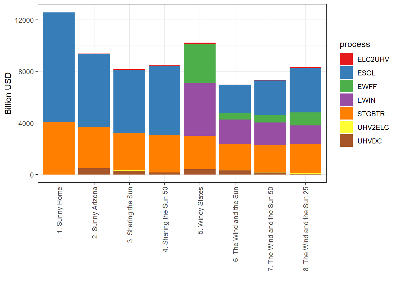
Total investments
code
# Technology investment
vTechInv <- getData(sns, name = "vTechInv", merge = T)

# Storage investment
vStorageInv <- getData(sns, name = "vStorageInv", merge = T)

# UHVDC grid investment
vTradeInv <- getData(sns, name = "vTradeInv", merge = T)

# All investments
vInvAll <- getData(sns, name_ = "Inv", merge = T, parameters = FALSE,
                   newNames = c("tech" = "process", "stg" = "process", "trade" = "process"))
# unique(vInvAll$name)
# unique(vInvAll$process)
ii <- grepl("^TRBD_", vInvAll$process)
# summary(ii)
vInvAll$process[ii] <- "UHVDC" # rename individual power lines
vInvAll <- vInvAll %>%
  group_by(scenario, process) %>%
  summarize(`Billion USD` = sum(value) / 1e3)

plt <- ggplot(vInvAll) +
  geom_bar(aes(x = scenario, y = `Billion USD`, fill = process),
           stat = "identity") +
  theme_bw() +
  theme(axis.text.x = element_text(angle = 90, hjust = 1, vjust = .5)) +
  scale_fill_brewer(palette = "Set1") +
  xlab("")
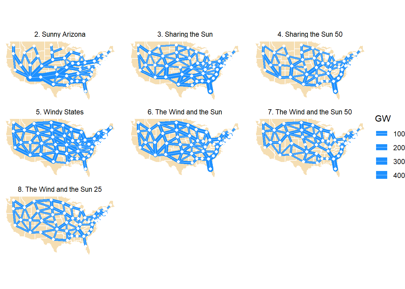
UHVDC grid structure
code
vTradeCap <- getData(sns, name = "vTradeCap", merge = T, newNames = c("value" = "GW")) %>%
  add_centers()

# ii <- grepl("SUNNYAZ", vTradeCap$scenario); summary(ii)
ii <- rep(TRUE, length(vTradeCap$scenario))

plt <- ggplot(data = usa49r) +
  geom_polygon(aes(x = long, y = lat, group = group), fill = "wheat",
               colour = "white", alpha = 1, size = .5) + # aes fill = id,
  coord_fixed(1.3) +
  guides(fill=FALSE) +  # off the color legend
  theme_void() +
  # labs(title = "Optimized UHV grid capacity")  +
  # theme(plot.title = element_text(hjust = 0.5),
  #       plot.subtitle = element_text(hjust = 0.5)) +
  geom_segment(aes(x=x.src, y=y.src, xend=x.dst, yend=y.dst, size = GW),
  # geom_segment(aes(x=xsrc, y=ysrc, xend=xdst, yend=ydst, size = GWh/1e3),
  # geom_segment(aes(x=xsrc, y=ysrc, xend=xdst, yend=ydst, size = GWh/1e2/8760),
               data = vTradeCap[ii,], inherit.aes = FALSE, #size = 3,
               alpha = 1, colour = "dodgerblue", lineend = "round", show.legend = T) +
  scale_size_continuous(range = c(1, 5)) +
  # , breaks = scales::breaks_pretty(5)(vTradeCap$GW)
  geom_segment(aes(x=x.src, y=y.src, xend=x.dst, yend=y.dst),
               data = vTradeCap[ii,], inherit.aes = FALSE, size = .1,
           # arrow = arrow(type = "closed", angle = 15,
           #               length = unit(0.15, "inches")),
           colour = "white", alpha = 0.75,
           lineend = "butt", linejoin = "mitre", show.legend = T) +
  geom_point(data = reg_centers, aes(x, y), colour = "white") +
  facet_wrap(~scenario, ncol = 3)

# ii <- grepl("SUNNYAZ", vTradeCap$scenario)
# ii <- ii & grepl("ND", vTradeCap$src) & grepl("SD", vTradeCap$dst)
# ii <- ii | (grepl("ND", vTradeCap$dst) & grepl("SD", vTradeCap$src))
# vTradeCap[ii,]
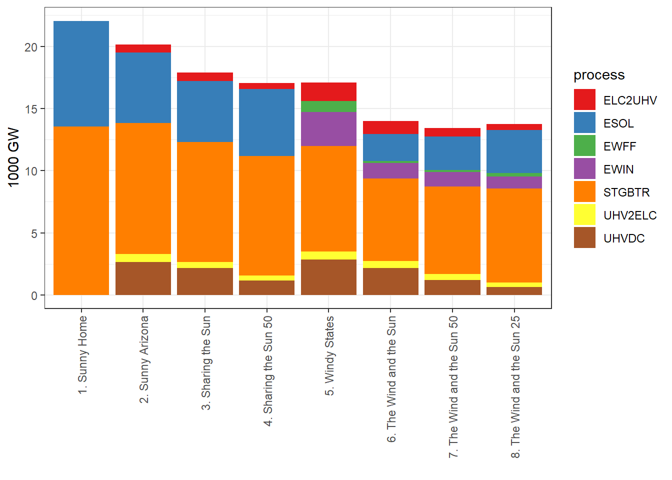
Capacity structure
code
vCap <- getData(sns, c("vTechCap", "vStorageCap"), merge = TRUE,
                newNames = c("tech" = "process", "stg" = "process", "trade" = "process")) %>%
  group_by(scenario, process) %>%
  summarise("GW" = sum(value))

vTradeCap_tot <-
  vTradeCap %>% group_by(scenario) %>%
  summarise(GW = sum(GW)) %>%
  mutate(process = "UHVDC")

vCap_tot <- full_join(vCap, vTradeCap_tot, by = names(vCap))

plt <- ggplot(vCap_tot) +
  geom_bar(aes(x = scenario, y = GW/1e3, fill = process),
           stat = "identity") +
  theme_bw() +
  theme(axis.text.x = element_text(angle = 90, hjust = 1, vjust = .5)) +
  scale_fill_brewer(palette = "Set1") +
  xlab("") + ylab("1000 GW")
Summary and discussion
The set of scenarios in the project evaluates a potential role of each source of renewable energy (solar, onshore and offshore wind) in the US electric power system. All of the scenarios assume exogenous demand, while the potential supply from renewables in each location (region) is also exogenous, defined by the historical weather. The only endogenous part (to be optimized by the model) is a way to balance the supply with the demand by means of choosing the location and capacity of generating technologies, energy storage, and power lines. The resulting (solved with minimal costs criteria) structure of the power sector depends on the available set of technologies and constraints which vary by scenarios.
The simulated from scratch states of the sector demonstrate the following known features of high-renewable power systems:
- importance of energy storage;
- importance of long-distance and well developed power network;
- curtailments.
The US-specific (based on the geography, the potential of renewables, costs, and allocation of demand) features, conclusions, observations:
- it is technically feasible to design an electric power system in the US, relying on just one source of intermittent renewable energy - solar or wind;
- the allocation of generating capacities may vary
- solar and wind energy resources have certain degree of complementarity, their combination may reduce overall system costs;
- solar energy is the dominant resource in all scenarios, the resource limit was not met (though actually available for the installation land was not considered);
- interregional power grid is an important technology for balancing intermittent resources across the country; constraints on investments to the network affect the capacity of individual power lines, though the constrained network still demonstrates connections of all regions, emphasizing the importance of the network expansion;
- all scenarios satisfy more than 99% of electric demand, except the only one which is not utilizing solar energy (“5. Windy States”), which was unable to deliver around 3.4% of electricity with marginal costs less that $10 USD/kWh.
- the reliability of the system is achieved by the over-capacity, which results high curtailment of supplied electricity (from 81% to 262%) of demanded electricity;
- systemwide costs of electricity generation varies from 5.8 to 9.5 cents/kWh across scenarios;
- considering the curtailments as the system losses, the systemwide costs of electricity varies from 12.7 US cents per kWh to 23 cents/kWh across scenarios.
While this exersise demonstrates possibility of 100% renewables-based electric power system in the US from the technical perspectives, the overcapacity and high curtailments make the overall design not very practical. In the considered simplified system, exogenous demand and supply put the main burden of the balancing on the distribution and energy storage. Consideration of additional balancing options, such as responsive demand, back-up generation capacities, may significantly reduce overcapacity and the overall system costs.