USENSYS - Electric Power Sector
Renewables balancing version (6.0) documentation (DRAFT)
Release notes
**Release notes:**
v6.0 (Apr 11, 2020)
– Rediced time resolution for supply commodities to improve performance.
– Added capacity constraints to control resource availability of solar and wind energy.v5.0 (Feb 22, 2020)
– Small adjustment according to the newer version of the energyRt package ().
– Investment costs of UHVDC lines increased (+50% for land, an assumption).
– Concevative storage costs for all scenarios.
– 100 interregional UHVDC power lines (vs. 80+ in previous version).
…
- v1.0 (May 4, 2019)
– First version. First set of scenarios.
– Exogenous trade routes.
## Loading required package: sp
## Loading required package: parallel
## Loading required package: ggplot2
##
##  Loading package: energyRt
##  Energy technology modeling toolbox in R
##  Version: 0.01.07.9000-beta (development version from GitHub)
##   <http://www.energyrt.org>
##
##
## Attaching package: 'lubridate'
## The following object is masked from 'package:base':
##
##     date
## -- Attaching packages --------------------------------------- tidyverse 1.3.0 --
## v tidyr   1.0.2     v dplyr   0.8.5
## v readr   1.3.1     v stringr 1.4.0
## v purrr   0.3.3     v forcats 0.5.0
## -- Conflicts ------------------------------------------ tidyverse_conflicts() --
## x lubridate::as.difftime() masks base::as.difftime()
## x lubridate::date()        masks base::date()
## x dplyr::filter()          masks stats::filter()
## x lubridate::intersect()   masks base::intersect()
## x dplyr::lag()             masks stats::lag()
## x lubridate::setdiff()     masks base::setdiff()
## x lubridate::union()       masks base::union()
Overview
The renewables balancing version of USENSYS (USENSYS_RENBAL) has a relatively high temporal resolution to better represent the potential of intermittent wind and solar power generation. Given hourly weather data by regions, the model optimizes the allocation of generating capacities, energy storage, long-distance electric power grid, and the structure of demand across regions based on minimal costs. The full year of hourly data (8760 hours) by 49 regions provide a good (for the capacity expansion class of models) approximation of a power system with intermittent resources. Though the additional granularity increases the computational burden. Therefore the model horizon is reduced to one year. Depending on scenario, the solution time varies from 1 to 24+ hours on 6-core, 5GHz Intel processor, 64Gb RAM, using GAMS/CPLEX.
The main features of the version of the model:
- 49 regions (48 lower states and District of Columbia);
- 1 year, 8760 hours (24x365);
- estimated demand for electricity in 2018 (monthly data by states, disaggregated by hours using national load curve - to be improved on further steps);
- Main technologies:
- solar PV arrays and wind farms,
- hourly electricity storage (>= 1 hour),
- seasonal electricity storage (>= 1 day),
- endogenous interregional grid (UHV power lines and converter stations),
- MERRA-2 weather data (see below the aggregation procedure);
- Demand options:
- fully exogenous demand (fixed in time and by regions),
- static demand with optimized location (fixed in time, endogenous location),
- time-shiftable demand within a day (24 calendar hours), fixed or optimized location,
- demand technologies with flexible consumption and restrictions on annual capacity utilization (“power-to-X”).
- Various policy and resource constraints.
The script below defines the model objects (regions, technologies, commodities, HVDC power lines, demand options, time resolution). The objects can be combined to define scenarios. The result of the entire script is saved in the data/USENSYS_RENBAL_v060.RData To change any parameters or costs, make the intended modification and rerun this script.
Map data
GIS information is used for evaluation of renewables potentials by the model regions, for estimation of distances between regions for electric power lines, and for graphical output.
Map objects:
usa49reg - lower 48 states + DC, spatial polygon data frame format;
usa49r - lower 48 states + DC, data frame format.
code
if (!file.exists(file.path(homedir, "data/maps/usa49reg.RData"))) {
  stop("US map data is not found. Follow the steps in 'usa_maps.R'")
} else {
  load(file.path(homedir, "data/maps/usa49reg.RData"))
}

b <- ggplot(usa49r, aes(long,lat, group = group, fill = id)) +
  geom_polygon(aes(fill = id), colour = rgb(1,1,1,.2)) +
  # geom_polygon(aes(fill = id), colour = "white", size = .75) +
  labs(fill = "Region") +
  coord_fixed(1.45) +
  # scale_fill_brewer(palette = "Paired") +
  #coord_quickmap() +
  theme_void() +
  theme(legend.position="none")

# Names of the regions in the model and the map-data
(reg_names <- unique(as.character(usa49reg@data$region)))
##  [1] "WA" "MT" "ME" "ND" "SD" "WY" "WI" "ID" "VT" "MN" "OR" "NH" "IA" "MA" "NE"
## [16] "NY" "PA" "CT" "RI" "NJ" "IN" "NV" "UT" "CA" "OH" "IL" "DC" "DE" "WV" "MD"
## [31] "CO" "KY" "KS" "VA" "MO" "AZ" "OK" "NC" "TN" "TX" "NM" "AL" "MS" "GA" "SC"
## [46] "AR" "LA" "FL" "MI"
(reg_names_in_gis <- as.character(usa49reg@data$region))
##  [1] "WA" "MT" "ME" "ND" "SD" "WY" "WI" "ID" "VT" "MN" "OR" "NH" "IA" "MA" "NE"
## [16] "NY" "PA" "CT" "RI" "NJ" "IN" "NV" "UT" "CA" "OH" "IL" "DC" "DE" "WV" "MD"
## [31] "CO" "KY" "KS" "VA" "MO" "AZ" "OK" "NC" "TN" "TX" "NM" "AL" "MS" "GA" "SC"
## [46] "AR" "LA" "FL" "MI"
# Number of regions
(nreg <- length(reg_names))
## [1] 49
(nreg_in_gis <- length(usa49reg@data$region))
## [1] 49
# Neighbor regions
nbr <- spdep::poly2nb(usa49reg)
names(nbr) <- usa49reg@data$region

# Geographic centers of the regions
reg_centers <- getCenters(usa49reg)

mobj <- c(mobj, "usa49r", "usa49reg", "reg_names", "reg_names_in_gis",
          "nreg", "nreg_in_gis", "nbr", "reg_centers")
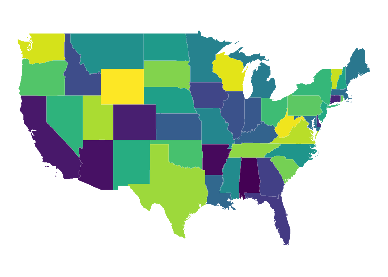
Figure 1: USENSYS regions.
Sub-annual time resolution (time-slices)
The sub-annual time in the model has two levels:
- the day of the year (YDAY), from 1 to 365;
- the hour (1 to 24).
The total number of time-slices (sub-annual time steps) is 8760. Every time-slice is named according to the format “dNNN_hNN”, where NNN - a day number in a year, NN - an hour in 24h format.
code
# A list with two levels slices
timeslices365 <- list(
  YDAY = paste0("d", formatC(1:365, width = 3, flag = "0")),
  HOUR = paste0("h", formatC(0:23, width = 2, flag = "0"))
)

# Function to convert data-time object into names of time-slices.
datetime2tsdh <- function(dt) {
  paste0("d", formatC(yday(dt), width = 3, flag = "0"), "_",
         "h", formatC(hour(dt), width = 2, flag = "0"))
}
# check
datetime2tsdh(today("EST"))
## [1] "d106_h00"
# Function to coerse time-slices names into data-time format, for a given year and time-zone.
tsdh2datetime <- function(tslice, year = 2018, tz = "EST") {
  DAY <- as.integer(substr(tslice, 2, 4)) - 1
  HOUR <- as.integer(substr(tslice, 7, 8))
  lubridate::ymd_h(paste0(year, "-01-01 0"), tz = tz) + days(DAY) + hours(HOUR)
}
# check
tsdh2datetime("d365_h23")
## [1] "2018-12-31 23:00:00 EST"
# data.frame object with names of the final time-slices in the model
#   and releted data-time information
slc365 <- tibble(
  slice = kronecker(timeslices365$YDAY, timeslices365$HOUR, FUN = "paste", sep = "_")
)
# add date-time info
slc365$syday <- substr(slc365$slice, 1, 4)
slc365$shour <- substr(slc365$slice, 6, 8)
slc365$yday <- as.integer(substr(slc365$slice, 2, 4))
slc365$hour <- as.integer(substr(slc365$slice, 7, 8))
slc365$datetime <- tsdh2datetime(slc365$slice)
slc365$month <- month(slc365$datetime)
slc365$week <- week(slc365$datetime)
head(slc365)
## # A tibble: 6 x 8
##   slice    syday shour  yday  hour datetime            month  week
##   <chr>    <chr> <chr> <int> <int> <dttm>              <dbl> <dbl>
## 1 d001_h00 d001  h00       1     0 2018-01-01 00:00:00     1     1
## 2 d001_h01 d001  h01       1     1 2018-01-01 01:00:00     1     1
## 3 d001_h02 d001  h02       1     2 2018-01-01 02:00:00     1     1
## 4 d001_h03 d001  h03       1     3 2018-01-01 03:00:00     1     1
## 5 d001_h04 d001  h04       1     4 2018-01-01 04:00:00     1     1
## 6 d001_h05 d001  h05       1     5 2018-01-01 05:00:00     1     1
tail(slc365)
## # A tibble: 6 x 8
##   slice    syday shour  yday  hour datetime            month  week
##   <chr>    <chr> <chr> <int> <int> <dttm>              <dbl> <dbl>
## 1 d365_h18 d365  h18     365    18 2018-12-31 18:00:00    12    53
## 2 d365_h19 d365  h19     365    19 2018-12-31 19:00:00    12    53
## 3 d365_h20 d365  h20     365    20 2018-12-31 20:00:00    12    53
## 4 d365_h21 d365  h21     365    21 2018-12-31 21:00:00    12    53
## 5 d365_h22 d365  h22     365    22 2018-12-31 22:00:00    12    53
## 6 d365_h23 d365  h23     365    23 2018-12-31 23:00:00    12    53
mobj <- c(mobj, "timeslices365", "datetime2tsdh", "tsdh2datetime", "slc365")
Commodities
Declaration of the model commodities.
code
ELC <- newCommodity(
  name = 'ELC',
  description = "Generic electricity",
  slice = "HOUR")
SOL <- newCommodity(
  name = 'SOL',
  description = "Solar energy",
  slice = "ANNUAL")
WIN <- newCommodity(
  name = 'WIN',
  description = "Wind energy, onshore",
  slice = "ANNUAL")
WFF <- newCommodity(
  name = 'WFF',
  description = "Wind energy, offshore",
  slice = "ANNUAL")
UHV <- newCommodity(
  name = 'UHV',
  description = "Ultra High Voltage electricity, DC",
  slice = "HOUR")
Demand
The final demand for electricity can be specifyed by hours as an exogenous load curve for each region of the model, or with temporal and/or spatial flexibility. The flexibility of demand might be achieved in several ways, as discussed below.
Exogenous load curve
Hourly demand by states (the curent version applies an aggregated national load curve for every region – to be updated with the actual consumption data).
code
eiadir <- file.path(file.path(homedir, "data/EIA"))
load(file.path(eiadir, "eia_raw.RData"))

# load curve data from:
# https://www.eia.gov/opendata/qb.php?sdid=EBA.US48-ALL.D.H
# Demand for United States Lower 48 (region), hourly - UTC time
lc <- read_csv(file.path(homedir,
                         "data/EIA/Demand_for_United_States_Lower_48_(region)_hourly_-_UTC_time.csv"),
               skip = 5, col_names = c("datetime", "MWh"))
## Parsed with column specification:
## cols(
##   datetime = col_character(),
##   MWh = col_double()
## )
dim(lc)
## [1] 40630 2
head(lc)
## # A tibble: 6 x 2
##   datetime          MWh
##   <chr>           <dbl>
## 1 02/18/2020 02H 470820
## 2 02/18/2020 01H 471417
## 3 02/18/2020 00H 463638
## 4 02/17/2020 23H 450007
## 5 02/17/2020 22H 441414
## 6 02/17/2020 21H 438162
lc$datetime_EST <- mdy_h(lc$datetime, tz = "EST")
lc$year <- year(lc$datetime_EST)
summary(lc$year)
##    Min. 1st Qu.  Median    Mean 3rd Qu.    Max.
##    2015    2016    2017    2017    2018    2020
lc <- lc[lc$year == 2018, ]
lc$slice <- datetime2tsdh(lc$datetime_EST)
lc <- lc[order(lc$datetime),]
lc$month <- month(lc$datetime_EST)
lc$hGWh <- lc$MWh/1e3

# Check
dim(lc)
## [1] 8760 7
lc
## # A tibble: 8,760 x 7
##    datetime         MWh datetime_EST         year slice    month  hGWh
##    <chr>          <dbl> <dttm>              <dbl> <chr>    <dbl> <dbl>
##  1 01/1/2018 00H 562684 2018-01-01 00:00:00  2018 d001_h00     1  563.
##  2 01/1/2018 01H 566264 2018-01-01 01:00:00  2018 d001_h01     1  566.
##  3 01/1/2018 02H 565612 2018-01-01 02:00:00  2018 d001_h02     1  566.
##  4 01/1/2018 03H 556869 2018-01-01 03:00:00  2018 d001_h03     1  557.
##  5 01/1/2018 04H 545727 2018-01-01 04:00:00  2018 d001_h04     1  546.
##  6 01/1/2018 05H 536422 2018-01-01 05:00:00  2018 d001_h05     1  536.
##  7 01/1/2018 06H 526434 2018-01-01 06:00:00  2018 d001_h06     1  526.
##  8 01/1/2018 07H 520531 2018-01-01 07:00:00  2018 d001_h07     1  521.
##  9 01/1/2018 08H 516766 2018-01-01 08:00:00  2018 d001_h08     1  517.
## 10 01/1/2018 09H 513790 2018-01-01 09:00:00  2018 d001_h09     1  514.
## # ... with 8,750 more rows
sum(lc$MWh) / 1e6
## [1] 4067.913
summary(lc$hGWh)
##    Min. 1st Qu.  Median    Mean 3rd Qu.    Max.
##   321.2   411.8   449.6   464.4   506.1   709.6
mlc <- group_by(lc, month) %>%
  summarise(mGWh = sum(MWh)/1e3)
loadcurve <- full_join(select(lc, datetime_EST, slice, hGWh, month), mlc)
## Joining, by = "month"
loadcurve$mshare <- loadcurve$hGWh / loadcurve$mGWh

# Check
group_by(loadcurve, month) %>%
  summarise(msum = sum(mshare))
## # A tibble: 12 x 2
##    month  msum
##    <dbl> <dbl>
##  1     1  1
##  2     2  1
##  3     3  1
##  4     4  1
##  5     5  1
##  6     6  1.00
##  7     7  1.00
##  8     8  1
##  9     9  1
## 10    10  1
## 11    11  1
## 12    12  1
# Filter unused data
elc_gen_2018 <- elc_gen[elc_gen$YEAR == 2018 &
                          elc_gen$`TYPE OF PRODUCER` ==
                          "Total Electric Power Industry" &
                          elc_gen$`ENERGY SOURCE` == "Total" &
                          elc_gen$STATE != "US-Total" &
                          elc_gen$STATE != "AK" &
                          elc_gen$STATE != "HI",]
elc_gen_2018
## # A tibble: 588 x 6
##     YEAR MONTH STATE `TYPE OF PRODUCER`    `ENERGY SOURCE` `GENERATION\r\n(Mega~
##    <dbl> <dbl> <chr> <chr>                 <chr>                           <dbl>
##  1  2018     1 AL    Total Electric Power~ Total                        13310533
##  2  2018     1 AR    Total Electric Power~ Total                         6177100
##  3  2018     1 AZ    Total Electric Power~ Total                         8208302
##  4  2018     1 CA    Total Electric Power~ Total                        14461936
##  5  2018     1 CO    Total Electric Power~ Total                         4681142
##  6  2018     1 CT    Total Electric Power~ Total                         3470117
##  7  2018     1 DC    Total Electric Power~ Total                            6937
##  8  2018     1 DE    Total Electric Power~ Total                          540139
##  9  2018     1 FL    Total Electric Power~ Total                        19687966
## 10  2018     1 GA    Total Electric Power~ Total                        12103582
## # ... with 578 more rows
sum(elc_gen_2018$`GENERATION\r\n(Megawatthours)`) / 1e6
## [1] 4161.304
sum(lc$MWh) / 1e6
## [1] 4067.913
length(unique(elc_gen_2018$STATE))
## [1] 49
elc_gen_2018$GWh <- elc_gen_2018$`GENERATION\r\n(Megawatthours)`/1e3
elc_gen_2018$month <- as.integer(elc_gen_2018$MONTH)
elc_gen_2018$region <- elc_gen_2018$STATE
elc_gen_2018 <- select(elc_gen_2018, month, region, GWh)

elc_gen_mhr <- full_join(loadcurve, elc_gen_2018)
## Joining, by = "month"
dim(elc_gen_mhr)[1]/49/365/24 == 1 # Check
## [1] TRUE
elc_gen_mhr$GWh <- elc_gen_mhr$GWh * elc_gen_mhr$mshare
sum(elc_gen_mhr$GWh); sum(lc$hGWh); sum(elc_gen_2018$GWh)
## [1] 4161304
## [1] 4067913
## [1] 4161304
# dim(elc_gen_mhr)
loadcurve <- select(elc_gen_mhr, -mGWh, -hGWh)
summary(loadcurve$GWh)
##     Min.  1st Qu.   Median     Mean  3rd Qu.     Max.
##  0.00368  4.02346  7.50708  9.69458 12.62367 88.11843
# Demand class
DEM_ELC_DH <- newDemand(
  name = "DEM_ELC_DH",
  description = "Fixed demand with load curve",
  commodity = "ELC",
  dem = data.frame(
    year = 2018,
    region = c(
      loadcurve$region),
    slice = c(
      loadcurve$slice),
    dem = round(loadcurve$GWh, 7)
    )
  # slice = "HOUR"
)

# Check
dim(DEM_ELC_DH@dem)
## [1] 429240 4
dim(DEM_ELC_DH@dem)[1] / 365 / 24
## [1] 49
summary(DEM_ELC_DH@dem$dem)
##     Min.  1st Qu.   Median     Mean  3rd Qu.     Max.
##  0.00368  4.02346  7.50708  9.69458 12.62367 88.11843
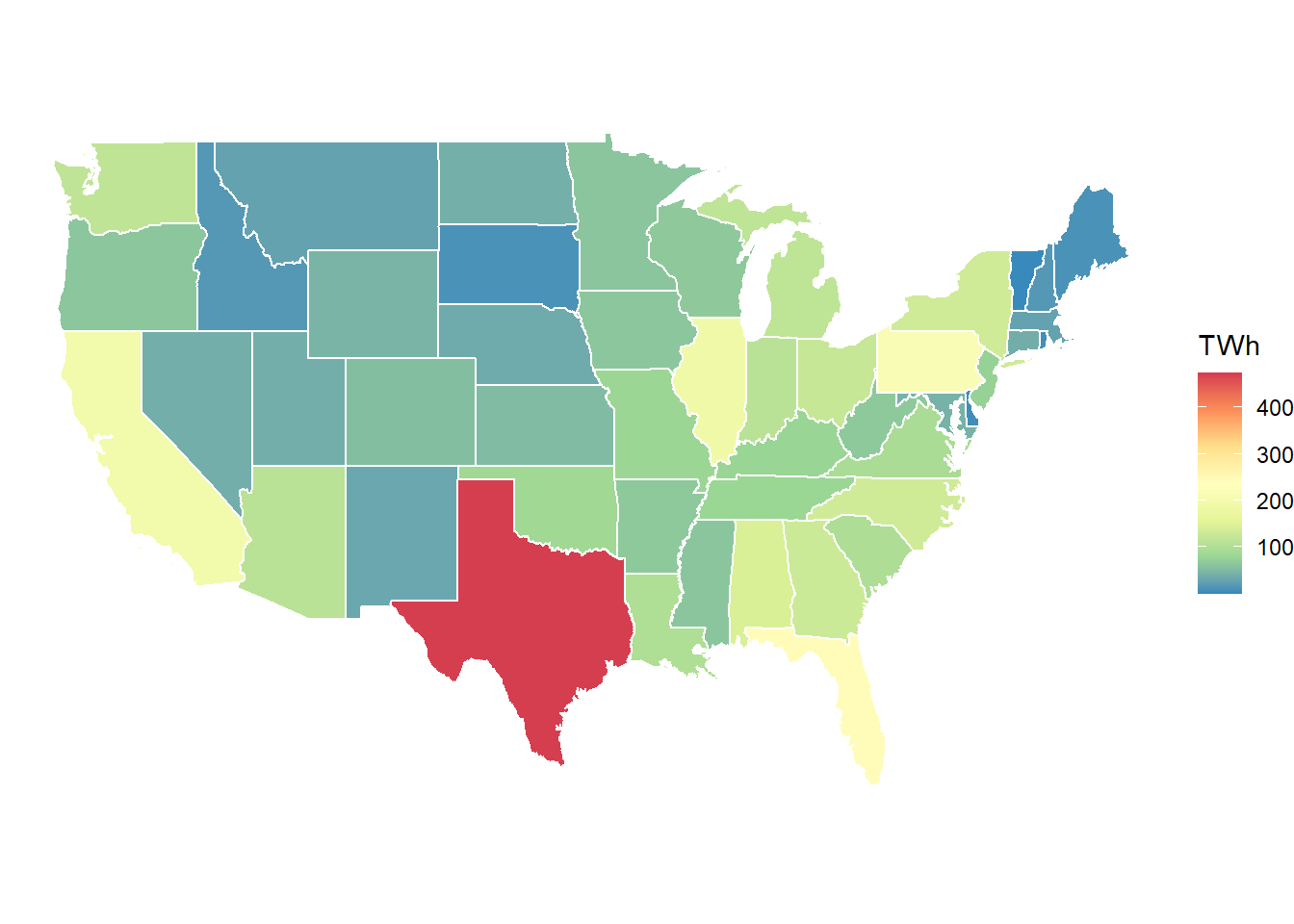
# Demand data for mapping
elc_gen_map <- elc_gen_2018 %>%
  group_by(region) %>%
  summarise(TWh = sum(GWh)/1e3) %>%
  full_join(usa49r, by = c("region" = "id"))
## Warning: Column `region`/`id` joining character vector and factor, coercing into
## character vector
elc_gen_map
## # A tibble: 11,481 x 8
##    region   TWh  long   lat order hole  piece group
##    <chr>  <dbl> <dbl> <dbl> <int> <lgl> <fct> <fct>
##  1 AL      145. -85.1  32.0     1 FALSE 1     AL.1
##  2 AL      145. -85.1  31.9     2 FALSE 1     AL.1
##  3 AL      145. -85.1  31.9     3 FALSE 1     AL.1
##  4 AL      145. -85.1  31.8     4 FALSE 1     AL.1
##  5 AL      145. -85.1  31.8     5 FALSE 1     AL.1
##  6 AL      145. -85.1  31.7     6 FALSE 1     AL.1
##  7 AL      145. -85.1  31.7     7 FALSE 1     AL.1
##  8 AL      145. -85.1  31.7     8 FALSE 1     AL.1
##  9 AL      145. -85.1  31.6     9 FALSE 1     AL.1
## 10 AL      145. -85.0  31.6    10 FALSE 1     AL.1
## # ... with 11,471 more rows
plt <- ggplot(elc_gen_map) +
  geom_polygon(aes(x = long, y = lat, group = group, fill = TWh), # fill = "wheat",
               colour = "white", alpha = 1, size = .5) +
  scale_fill_distiller(palette = "Spectral") +
  coord_fixed(1.45) +
  theme_void()

# ggsave(filename = "fig/elc_gen_map.png", plot = plt)
“Flat” load curve
code
elc_dem_fx <- loadcurve #
elc_dem_fx$year <- USENSYS$modelYear

for (y in unique(elc_dem_fx$year)) {
  for (r in reg_names) {
    ii <- elc_dem_fx$year == y & elc_dem_fx$region == r
    elc_dem_fx$GWh[ii] = mean(elc_dem_fx$GWh[ii]) # make it constant for each region and year
  }
}
# elc_dem_fx$PJ <- convert("GWh", "PJ", elc_dem_fx$GWh)
# elc_dem_fx

# Technology for flexible demand within a year, with minimal annual load
DEM_ELC_FX <- newDemand(
  name = "DEM_ELC_FX",
  description = "Flat, fixed demand",
  commodity = "ELC",
  dem = list(
    year = elc_dem_fx$year,
    region = elc_dem_fx$region,
    slice = elc_dem_fx$slice,
    dem = elc_dem_fx$GWh
    )
)
dim(DEM_ELC_FX@dem)
## [1] 429240 4
unique(DEM_ELC_FX@dem$year)
## [1] 2018
length(unique(DEM_ELC_FX@dem$region))
## [1] 49
length(unique(DEM_ELC_FX@dem$slice))
## [1] 8760
elc_dem_fx_reg_y <- elc_dem_fx %>%
  group_by(region, year) %>%
  summarise(GWh = sum(GWh))
elc_dem_fx_reg_y
## # A tibble: 49 x 3
## # Groups:   region [49]
##    region  year      GWh
##    <chr>  <int>    <dbl>
##  1 AL      2018 144989.
##  2 AR      2018  67134.
##  3 AZ      2018 112303.
##  4 CA      2018 197227.
##  5 CO      2018  56010.
##  6 CT      2018  39042.
##  7 DC      2018     79.5
##  8 DE      2018   6014.
##  9 FL      2018 244898.
## 10 GA      2018 130061.
## # ... with 39 more rows
elc_dem_fx_y_GWh <- sum(elc_dem_fx_reg_y$GWh)
elc_dem_fx_y_GWh
## [1] 4161304
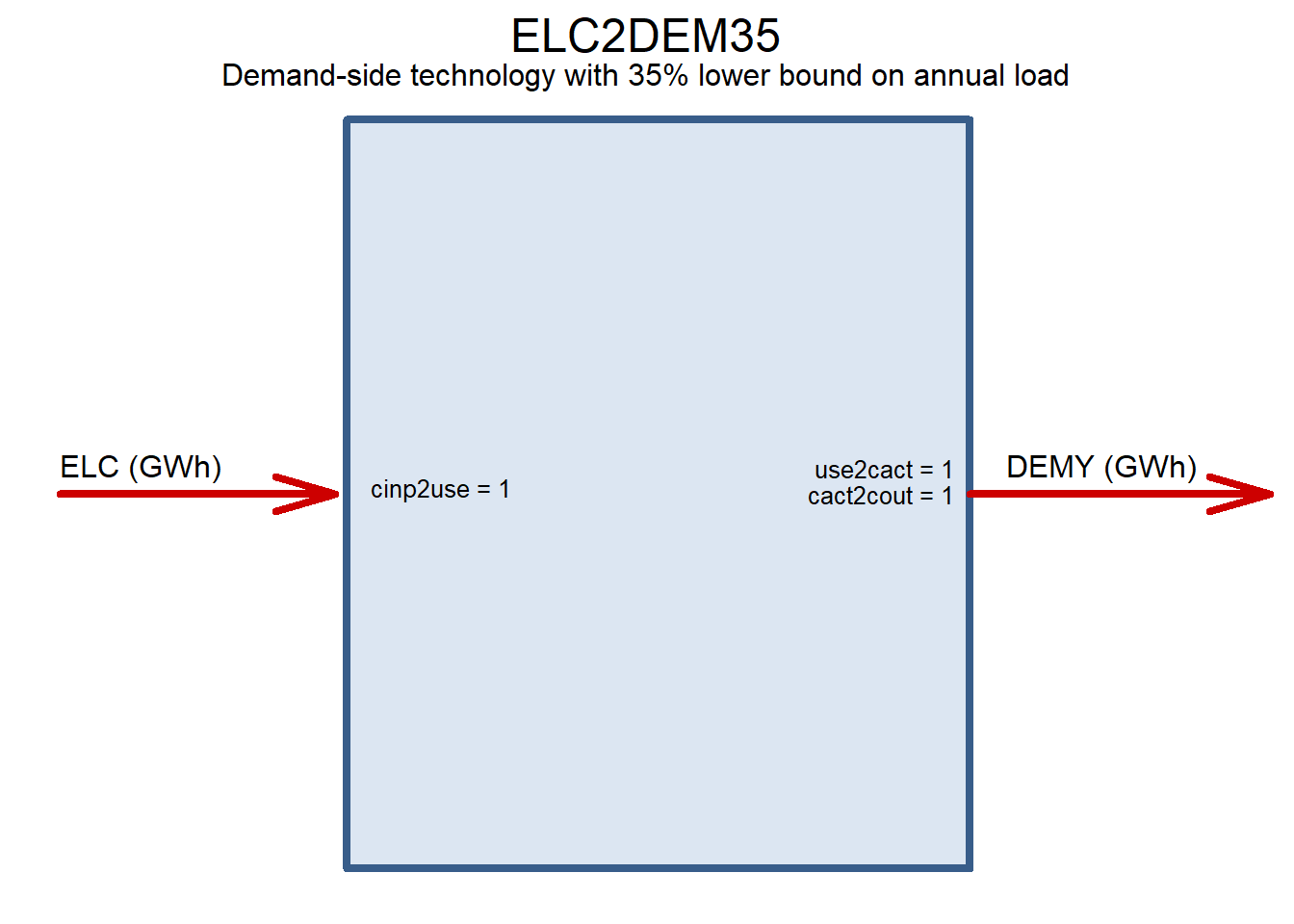
Demand-side technology with flexible load
Any technology with seasonally and hourly flexible load, for example Power-to-X (P2X).
code
DEM35 <- newCommodity(
  "DEM35",
  description = "",
  slice = "HOUR")

ELC2DEM35 <- newTechnology(
  name = "ELC2DEM35",
  description = "Demand-side technology with 35% lower bound on annual load",
  # region = reg_names,
  input = list(
    comm = "ELC",
    unit = "GWh"
  ),
  output = list(
    # comm = "DEM35",
    comm = "DEMY",
    unit = "GWh"
  ),
  cap2act = 24*365,
  afs = list(
    slice = "ANNUAL",
# The technology cannot have less than 35% annual load (in each region)
    afs.lo = .35
  ),
  # invcost = list(
  #   invcost = 1 # arbitrary small number for tracking
  # ),
  varom = list(varom = convert("cents/kWh", "MUSD/GWh", 10)),
  # olife = list(olife = 100),
  slice = "HOUR"
)
draw(ELC2DEM35)
ELC2DEM35CAP <- newConstraintS(
  name = "ELC2DEM35CAP",
  eq = ">=",
  type = "capacity",
  for.each = list(
    year = USENSYS$modelYear,
    tech = "ELC2DEM35"),
  for.sum = list(
    region = reg_names
  ),
  rhs = round(elc_dem_fx_y_GWh / 24 / 365 * 0.25)) # limit on capacity

DEM35EXP <- newExport(
  name = "DEM35EXP",
  description = "Annual demand for technologies with 35% annual load",
  commodity = "DEM35",
  exp = list(
    price = convert("cents/kWh", "MUSD/GWh", 1) # sell for 1 cent
  )
)
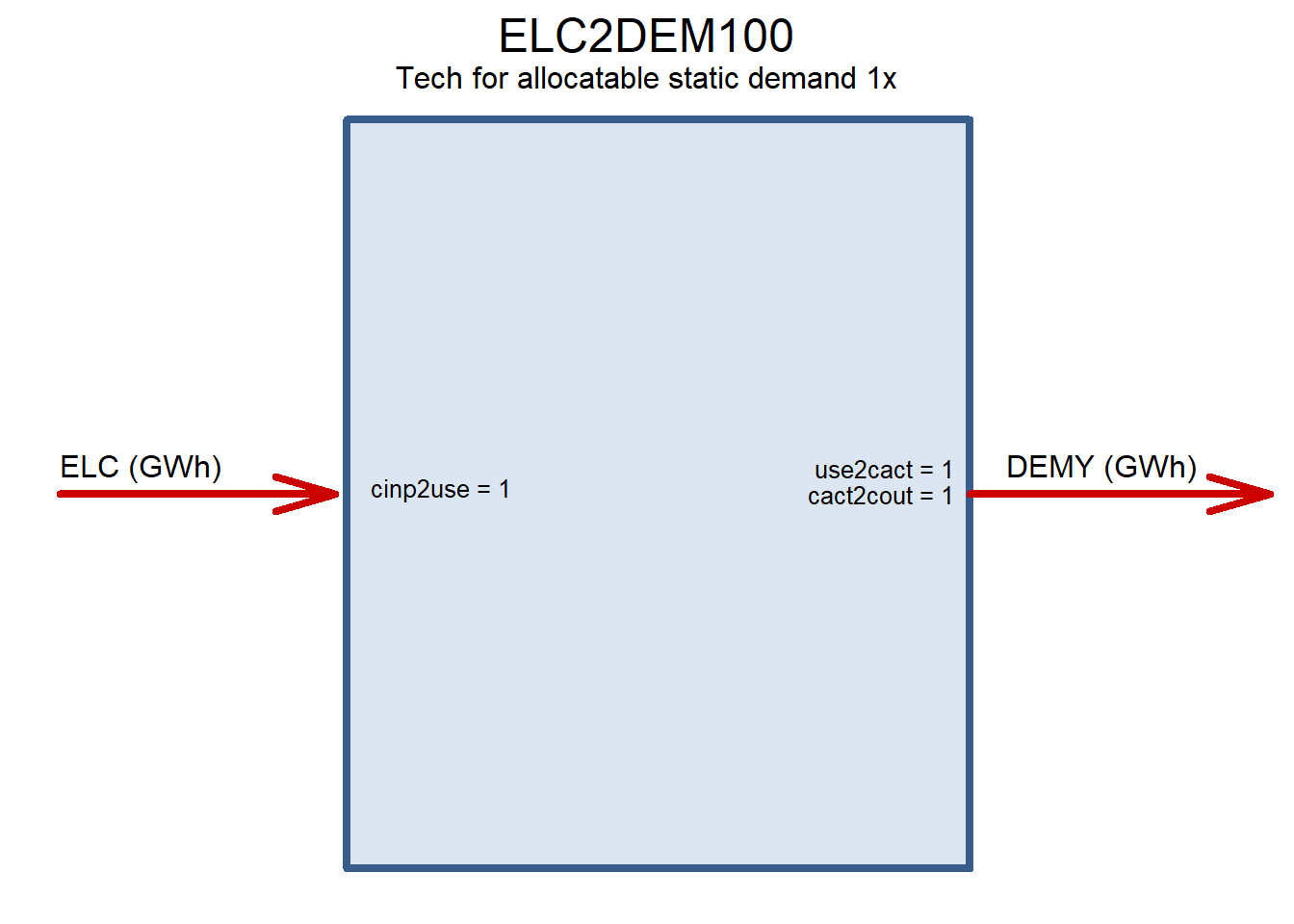
Optimized location
code
DEM100 <- newCommodity("DEM100", slice = "HOUR")

DEMY <- newCommodity("DEMY", slice = "ANNUAL")

ELC2DEM100 <- newTechnology(
  name = "ELC2DEM100",
  description = "Tech for allocatable static demand 1x",
  input = list(
    comm = "ELC",
    unit = "GWh"
    # unit = "PJ"
  ),
  output = list(
    # comm = "DEM100",
    comm = "DEMY",
    unit = "GWh"
    # unit = "PJ"
  ),
  cap2act = 24*365,
  # afs = list(
  #   slice = "ANNUAL",
  #   afs.lo = 1
  # ),
  af = list(
    af.lo = 1
  ),
  slice = "HOUR"
)
draw(ELC2DEM100)
CELC2DEM100CAPFX <- newConstraintS(
  name = "CELC2DEM100CAPFX",
  eq = ">=",
  type = "capacity",
  for.each = list(
    year = 2018,
    tech = "ELC2DEM100"),
  for.sum = list(
    region = reg_names
  ),
  rhs = round(elc_dem_fx_y_GWh / 24 / 365 * .5)) # limit on capacity

CELC2DEM100CAPUP <- newConstraintS(
  name = "CELC2DEM100CAPUP",
  eq = "<=",
  type = "capacity",
  for.each = list(
    year = 2018,
    region = reg_names,
    tech = "ELC2DEM100"),
  rhs = CELC2DEM100CAPFX@defVal/10) # at least 10 regions


DEM100DEXP <- newExport(
  name = "DEM100DEXP",
  description = "Flexible demand",
  commodity = "DEM100",
  exp = list(
    price = convert("cents/kWh", "MUSD/GWh", 10) # sell for 1 cent
  )
)
Intraday, 24h flexible demand (DSM)
code
DSMD <- newCommodity("DSMD", slice = "YDAY")

ELC2DSMD <- newTechnology(
  name = "ELC2DSMD",
  description = "Tech to convert ELC from HOUR to YDAY",
  input = list(
    comm = "ELC",
    unit = "GWh"
    # unit = "PJ"
  ),
  output = list(
    # comm = "DSMD",
    comm = "DEMY",
    unit = "GWh"
    # unit = "PJ"
  ),
  # cap2act = 31.536, #convert("GWh", "PJ", 24 * 365),
  cap2act = 24*365,
  afs = list(
    # slice = "MONTH",
    slice = timeslices365$YDAY,
# # The technology should be x% operational in every region where exists
# # < 1 allows some seasonality if export-demand is used for DSMD,
# # but should't affect anything if demand is used for DSMD
    afs.lo = rep(9/24, length(timeslices365$YDAY))
  ),
  # invcost = list(
  #   invcost = 1 # arbitrary small number for tracking
  # )
  # varom = list(varom = convert("USD/kWh", "MUSD/PJ", .01)),
  varom = list(varom = convert("cents/kWh", "MUSD/GWh", 5)),
  # stock = data.frame(
  #   region = elc_dem_fx_reg_y$region,
  #   stock = elc_dem_fx_reg_y$GWh/365/24 * 0.25 # 25% additional to the static demand
  # ),
  # end = list(
  #   end = 2010
  # ),
  slice = "HOUR"
)
# ELC2DSMD@stock$stock <- ELC2DSMD@stock$stock / ELC2DSMD@afs$afs.lo[1] # Adjust capacity
draw(ELC2DSMD)

# DSMDEXP <- newExport(
#   name = "DSMDEXP",
#   description = "Flexible demand",
#   commodity = "DSMD",
#   exp = list(
#     price = convert("cents/kWh", "MUSD/GWh", 5) # sell for 1 cent
#   )
# )
#
elc_gen_2018_reg_y <- elc_gen_2018 %>%
  group_by(region) %>%
  summarise(GWh = sum(GWh))


DEMYEXP <- newExport(
  name = "DEMYEXP",
  # description = "Flexible demand",
  commodity = "DEMY",
  exp = data.frame(
    slice = "ANNUAL",
    region = elc_gen_2018_reg_y$region,
    # exp.up = elc_gen_2018_reg_y$GWh,
    exp.fx = elc_gen_2018_reg_y$GWh,
    price = convert("cents/kWh", "MUSD/GWh", 15)
  )
)
Weather factors
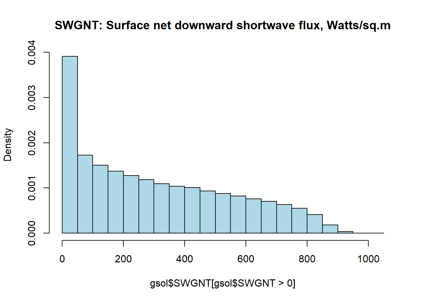
Hourly weather information is used to estimate the output of intermittent renewables, solar PVs and wind tourbines. The weather information is supplied as multipliers to availability factors of the generating technologies. I.e. availability of solar energy can be estimated based on the solar radiation (flux) data, or actual output of the technology (PV) expected under complex weather data (direct and indirect solar irradience, temperature, and/or clouds etc.). The estimation can be done on grid data, then aggregated using potentially perspective and available locations for the installation of the sollar arrays. Here, for simplicity, we estimate availability of the solar resource based on NASA’s “surface net downward shortwave flux” (SWGNT, Watts per square meter), assuming that the full capacity of PV arrays is achieved at 800 W/m2 level of the flux. This estimate is certainly not the best one, can be improved.
The estimated factors are aggregated for all availabel locations by states (which implies that allocation of PVs capacity is assumed to be evenly distributed across all the therritory in each state).
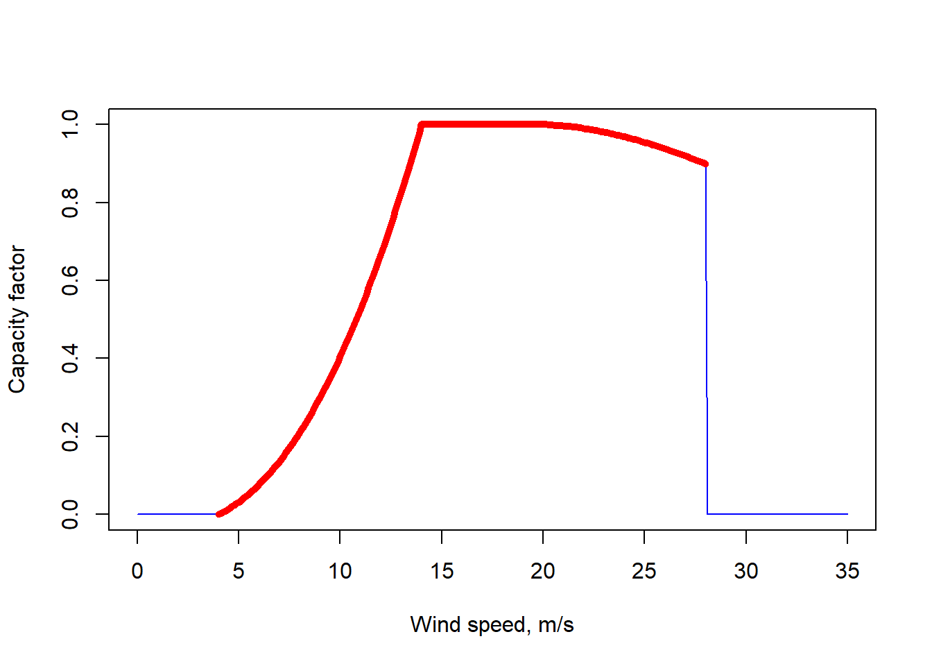
For wind energy, wind-power curves are used to estimate potential output of wind-mills across locations with the best potential of wind energy.
Land assumptions based on MERRA-2 data
1 degree of lattitude is about 111 km | x 0.625 = ~ 69 km
1 degree of latitude at ~20-50 degree is ~100-70km | * 0.5 = ~35-50km
1 cell of NASA grid is from 3569 to 5069 == 2415 (North) to 3450 (South) sq.km
we can take 3000 sq.km as approximation for all locations
Solar availability factors
code
Land requirements for solar PVs
1sq.m PV requires ~2.5sq.m of land
1.046 * 1.558 PV panel 345 Watt / 1.63 m2 ~= 200 Watt/m2 == .2 GW/km^2 /2.5 = .08 GW/km^2 = 80GW/1000km^2
Spacing ~ .08 GW per sq.km assuming PV efficiency = 0.2
Increase pf PV efficiency will require less space (0.08 * 1.5 = 0.12GW for 30% efficiency and 0.16GW for 40% PV efficiency)
# Share of land in every region which potentially can be used for PVs:
PV_coverage_share_max <- 0.1 # an assumption (almost unrestricted case)
PV_GW_max <- .08 * 3000 * PV_coverage_share_max # per one MERRA-2 grid cell

# MERRA-2 data:
# https://gmao.gsfc.nasa.gov/reanalysis/MERRA-2/data_access/
# here we use data for one year only
load(file.path(homedir, "data/MERRA2/nasa_sol_US49.RData"))
gsol
## # A tibble: 22,916,160 x 11
##    datetime            loc_id SWGDN SWGNT   lon   lat region  hour month mdays
##    <dttm>               <int> <dbl> <dbl> <dbl> <dbl> <fct>  <int> <fct> <int>
##  1 2017-01-01 00:30:00 133216     0     0 -80.6  25.5 FL         0 Janu~    31
##  2 2017-01-01 00:30:00 133765     0     0 -97.5  26   TX         0 Janu~    31
##  3 2017-01-01 00:30:00 133791     0     0 -81.2  26   FL         0 Janu~    31
##  4 2017-01-01 00:30:00 133792     0     0 -80.6  26   FL         0 Janu~    31
##  5 2017-01-01 00:30:00 134339     0     0 -98.8  26.5 TX         0 Janu~    31
##  6 2017-01-01 00:30:00 134340     0     0 -98.1  26.5 TX         0 Janu~    31
##  7 2017-01-01 00:30:00 134341     0     0 -97.5  26.5 TX         0 Janu~    31
##  8 2017-01-01 00:30:00 134366     0     0 -81.9  26.5 FL         0 Janu~    31
##  9 2017-01-01 00:30:00 134367     0     0 -81.2  26.5 FL         0 Janu~    31
## 10 2017-01-01 00:30:00 134368     0     0 -80.6  26.5 FL         0 Janu~    31
## # ... with 22,916,150 more rows, and 1 more variable: yday <dbl>
summary(gsol$SWGNT)
##     Min.  1st Qu.   Median     Mean  3rd Qu.     Max.
##    0.000    0.000    7.051  167.446  294.875 1011.000
hist(gsol$SWGNT[gsol$SWGNT > 0], col = "lightblue", probability = T,
     main = "SWGNT: Surface net downward shortwave flux, Watts/sq.m")
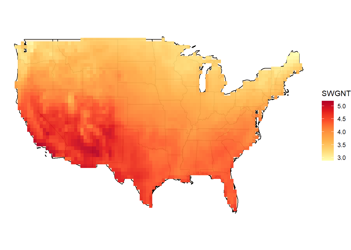
# Annual aggregate, kWh/day
ysol <- group_by(gsol, loc_id, lat, lon, region) %>%
  summarise(SWGNT = sum(SWGNT)/365/1e3)

# Max capacity by MERRA-2 locations
PV_GW_max_reg <- ysol %>%
  group_by(region) %>%
  summarise(GW_up = PV_GW_max * n())

ggplot(usa49r, aes(long, lat, group = group)) +
  geom_polygon(colour = "black", fill = "wheat", alpha = .5) +
  coord_fixed(1.45) +
  theme_void() +
  geom_raster(data = ysol, aes(lon, lat, fill = SWGNT), interpolate = F, inherit.aes = F, alpha = .95) +
  scale_fill_distiller(palette = "YlOrRd", direction = 1)
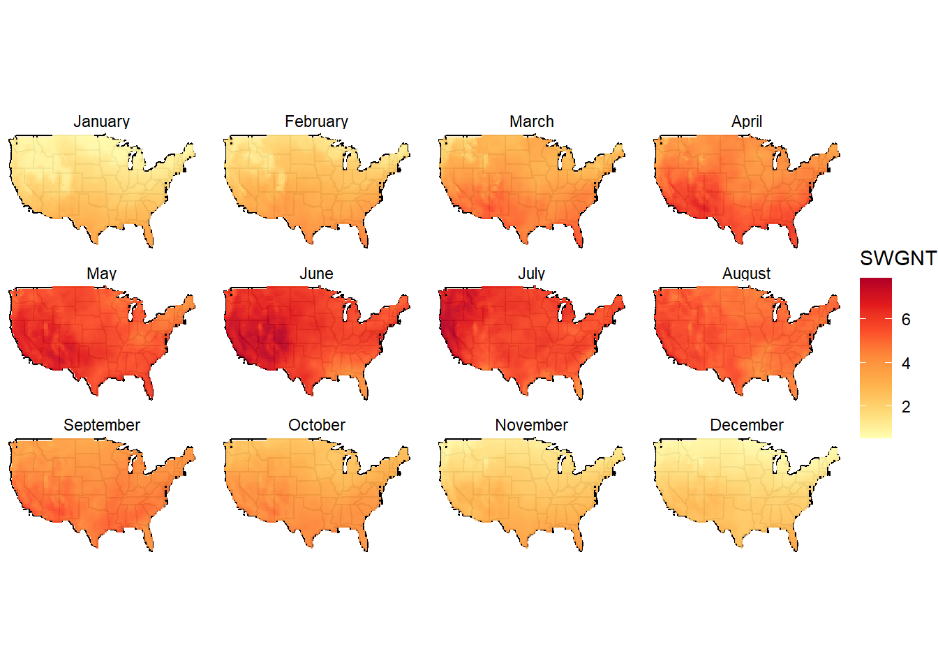
# By months, kWh/day
msol <- group_by(gsol, loc_id, lat, lon, region, month) %>%
  summarise(SWGNT = sum(SWGNT/mdays)/1e3)

ggplot(usa49r, aes(long, lat, group = group)) +
  geom_polygon(colour = "black", fill = "wheat", alpha = .5) +
  coord_fixed(1.45) +
  theme_void() +
  geom_raster(data = msol, aes(lon, lat, fill = SWGNT), interpolate = F, inherit.aes = F, alpha = .95) +
  scale_fill_distiller(palette = "YlOrRd", direction = 1) +
  facet_wrap(.~month)
# Aggregation regions
dhsol <- group_by(gsol, region, yday, hour) %>% # lat, lon,
  summarise(SWGNT = mean(SWGNT))
summary(dhsol$SWGNT)
##    Min. 1st Qu.  Median    Mean 3rd Qu.    Max.
##   0.000   0.000   7.611 162.951 291.846 937.517
# Estimated weather factors
dhsol$WF <- dhsol$SWGNT / 800
dhsol$WF[dhsol$WF > 1] <- 1
dhsol$WF[dhsol$WF < .03] <- 0 # kick-starting irradiance
summary(dhsol$WF)
##    Min. 1st Qu.  Median    Mean 3rd Qu.    Max.
##  0.0000  0.0000  0.0000  0.2025  0.3648  1.0000
dhsol
## # A tibble: 420,480 x 5
## # Groups:   region, yday [17,520]
##    region  yday  hour  SWGNT     WF
##    <fct>  <dbl> <int>  <dbl>  <dbl>
##  1 AL         1     0  0     0
##  2 AL         1     1  0     0
##  3 AL         1     2  0     0
##  4 AL         1     3  0     0
##  5 AL         1     4  0     0
##  6 AL         1     5  0     0
##  7 AL         1     6  0     0
##  8 AL         1     7  0.281 0
##  9 AL         1     8 23.9   0
## 10 AL         1     9 75.4   0.0942
## # ... with 420,470 more rows
# Add slice-names
dhsol$slice <- paste0("d", formatC(dhsol$yday, width = 3, flag = "0"),
                      "_h", formatC(dhsol$hour, width = 2, flag = "0"))
dhsol
## # A tibble: 420,480 x 6
## # Groups:   region, yday [17,520]
##    region  yday  hour  SWGNT     WF slice
##    <fct>  <dbl> <int>  <dbl>  <dbl> <chr>
##  1 AL         1     0  0     0      d001_h00
##  2 AL         1     1  0     0      d001_h01
##  3 AL         1     2  0     0      d001_h02
##  4 AL         1     3  0     0      d001_h03
##  5 AL         1     4  0     0      d001_h04
##  6 AL         1     5  0     0      d001_h05
##  7 AL         1     6  0     0      d001_h06
##  8 AL         1     7  0.281 0      d001_h07
##  9 AL         1     8 23.9   0      d001_h08
## 10 AL         1     9 75.4   0.0942 d001_h09
## # ... with 420,470 more rows
dim(dhsol)[1] / 365/24 # 48, i.e. one region is missing - DC
## [1] 48
dhsol$region <- as.character(dhsol$region)
reg_names[!(reg_names %in% unique(dhsol$region))]
## [1] "DC"
# Use MD weather data for DC
dhsol_DC <- dhsol[dhsol$region == "MD",]
dim(dhsol_DC)
## [1] 8760 6
dhsol_DC$region <- "DC"
dhsol_DC
## # A tibble: 8,760 x 6
## # Groups:   region, yday [365]
##    region  yday  hour SWGNT    WF slice
##    <chr>  <dbl> <int> <dbl> <dbl> <chr>
##  1 DC         1     0   0   0     d001_h00
##  2 DC         1     1   0   0     d001_h01
##  3 DC         1     2   0   0     d001_h02
##  4 DC         1     3   0   0     d001_h03
##  5 DC         1     4   0   0     d001_h04
##  6 DC         1     5   0   0     d001_h05
##  7 DC         1     6   0   0     d001_h06
##  8 DC         1     7  10.8 0     d001_h07
##  9 DC         1     8  96.1 0.120 d001_h08
## 10 DC         1     9 202.  0.253 d001_h09
## # ... with 8,750 more rows
# Add DC
dhsol <- bind_rows(dhsol, dhsol_DC)
dim(dhsol)[1] / 365/24
## [1] 49
length(unique(dhsol$region)) == nreg # double-check
## [1] TRUE
size(gsol); rm(gsol)
## [1] "1.5 Gb"
Wind availability factors
code
# Hourly wind speed data at 50 meters height for US, 2018
# (source: NASA/MERRA2, preprocessed)
load(file.path(homedir, "data/merra2/nasa_wnd_US49.RData"))
gwnd
## # A tibble: 26,481,480 x 19
##    datetime            loc_id WS50M   lon   lat US_100km_buffer US_10km_buffer
##    <dttm>               <int> <dbl> <dbl> <dbl> <lgl>           <lgl>
##  1 2017-01-01 00:30:00 132062  7.46 -81.9  24.5 TRUE            FALSE
##  2 2017-01-01 00:30:00 132063  7.67 -81.2  24.5 TRUE            FALSE
##  3 2017-01-01 00:30:00 132064  7.78 -80.6  24.5 TRUE            FALSE
##  4 2017-01-01 00:30:00 132065  7.92 -80    24.5 TRUE            FALSE
##  5 2017-01-01 00:30:00 132638  6.98 -81.9  25   TRUE            FALSE
##  6 2017-01-01 00:30:00 132639  6.93 -81.2  25   TRUE            FALSE
##  7 2017-01-01 00:30:00 132640  7.43 -80.6  25   TRUE            TRUE
##  8 2017-01-01 00:30:00 132641  7.82 -80    25   TRUE            FALSE
##  9 2017-01-01 00:30:00 132642  7.98 -79.4  25   TRUE            FALSE
## 10 2017-01-01 00:30:00 133213  6.70 -82.5  25.5 TRUE            FALSE
## # ... with 26,481,470 more rows, and 12 more variables: non_US <lgl>,
## #   drop <lgl>, US_land <lgl>, offshore <lgl>, nearest_neighbor <chr>,
## #   region <fct>, buff_10km <chr>, offshore_names <chr>, hour <int>,
## #   month <fct>, mdays <int>, yday <int>
if (is.factor(gwnd$region)) gwnd$region <- as.character(gwnd$region)

# Simplified aggregated wind-power curve as a function of wind speed.
# (assumed, should be replaced by read)
WindPowerCurve <- function(x = NULL,
                           xcutin = 4, xpeak = 14, xpeak2 = 20, xcutoff = 28,
                           ycutoff = .9, round = 3) {
  # x - wind speed in m/s
  # xcutin, xcutoff - operational speed of wind (m/s, min and max respectively)
  # xpeak, xpeak2 - the range of speed of with peak (nameplate) power
  # ycutoff - output factor at cut off (max) wind speed
  ff1 <- function(x1) {
    xx <- c(xcutin, 0.5 * (xpeak + xcutin), xpeak)
    xx2 <- xx * xx
    xx3 <- xx * xx2
    yy <- c(0, .3, 1)
    ff <- lm(yy ~ 0 + xx + xx + xx2 + xx3)
    predict(ff, data.frame(
      xx = x1,
      xx2 = x1 * x1,
      xx3 = x1 * x1 * x1
    ))
  }
  ff2 <- function(x2) {
    xx <- c(xpeak2, 0.5 * (xcutoff + xpeak2), xcutoff)
    xx2 <- xx * xx
    xx3 <- xx * xx2
    yy <- c(1, .51 * (ycutoff + 1), ycutoff)
    ff <- lm(yy ~ 0 + xx + xx + xx2 + xx3)
    predict(ff, data.frame(
      xx = x2,
      xx2 = x2 * x2,
      xx3 = x2 * x2 * x2
    ))
  }
  y <- rep(0., length(x))
  ii <- x <= xcutin
  y[ii] <- 0
  ii <- x > xcutoff
  y[ii] <- 0
  ii <- x >= xpeak & x <= xpeak2
  y[ii] <- 1
  ii <- x > xcutin & x < xpeak
  y[ii] <- ff1(x[ii])
  ii <- x > xpeak2 & x <= xcutoff
  y[ii] <- ff2(x[ii])
  return(round(y, round))
  # splinefun(xx, yy, method = "natural")
}

# Check
WindPowerCurve(0:30)
##  [1] 0.000 0.000 0.000 0.000 0.000 0.031 0.077 0.136 0.210 0.300 0.406 0.528
## [13] 0.667 0.825 1.000 1.000 1.000 1.000 1.000 1.000 1.000 0.997 0.990 0.981
## [25] 0.969 0.955 0.938 0.920 0.900 0.000 0.000
x <- seq(0, 35, by = .1)
plot(x, WindPowerCurve(x), type = "l", col = "blue", lwd = 1,
     xlab = "Wind speed, m/s", ylab = "Capacity factor")
x1 <- seq(4, 28, by = .1)
points(x1, WindPowerCurve(x1), type = "l", col = "red", lwd = 5)
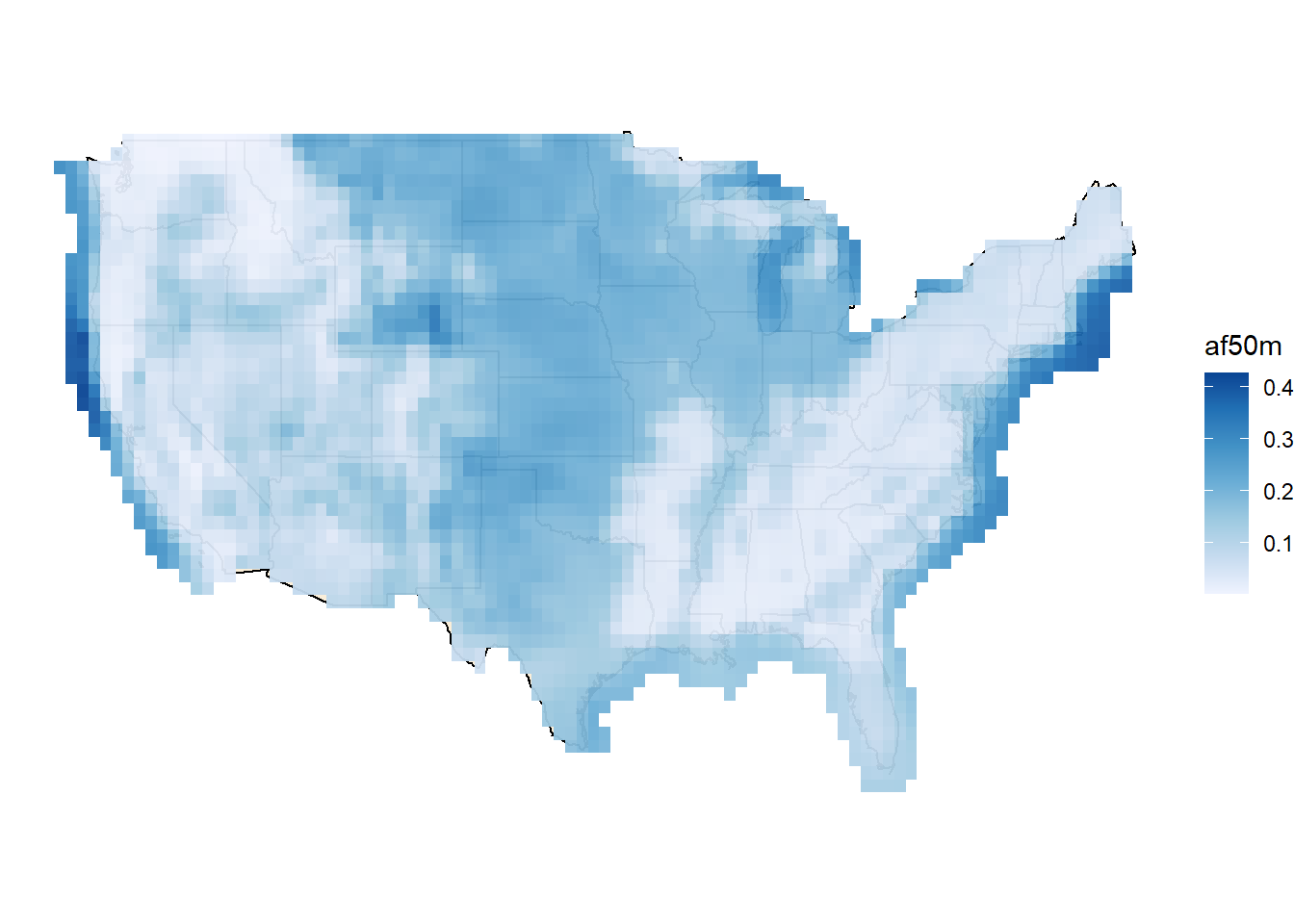
# Availability factor for wind-energy technologies,
# estimated based on the wind-power curve
gwnd$af50m <- WindPowerCurve(gwnd$WS50M)

# Annual availability factor of wind turbines by location
ywnd <- group_by(gwnd, loc_id, lat, lon, region) %>%
  summarise(af50m = sum(af50m)/365/24)

ggywnd <- function(ii = rep(T, length(ywnd$loc_id))) {
  ggplot(usa49r, aes(long,lat, group = group)) +
    geom_polygon(colour = "black", fill = "wheat", alpha = .5) +
    coord_fixed(1.45) +
    theme_void() +
    geom_raster(data = ywnd[ii,], aes(lon, lat, fill = af50m),
                interpolate = F, inherit.aes = F, alpha = .95) +
    scale_fill_distiller(palette = "Blues", direction = 1)
}
ggywnd()
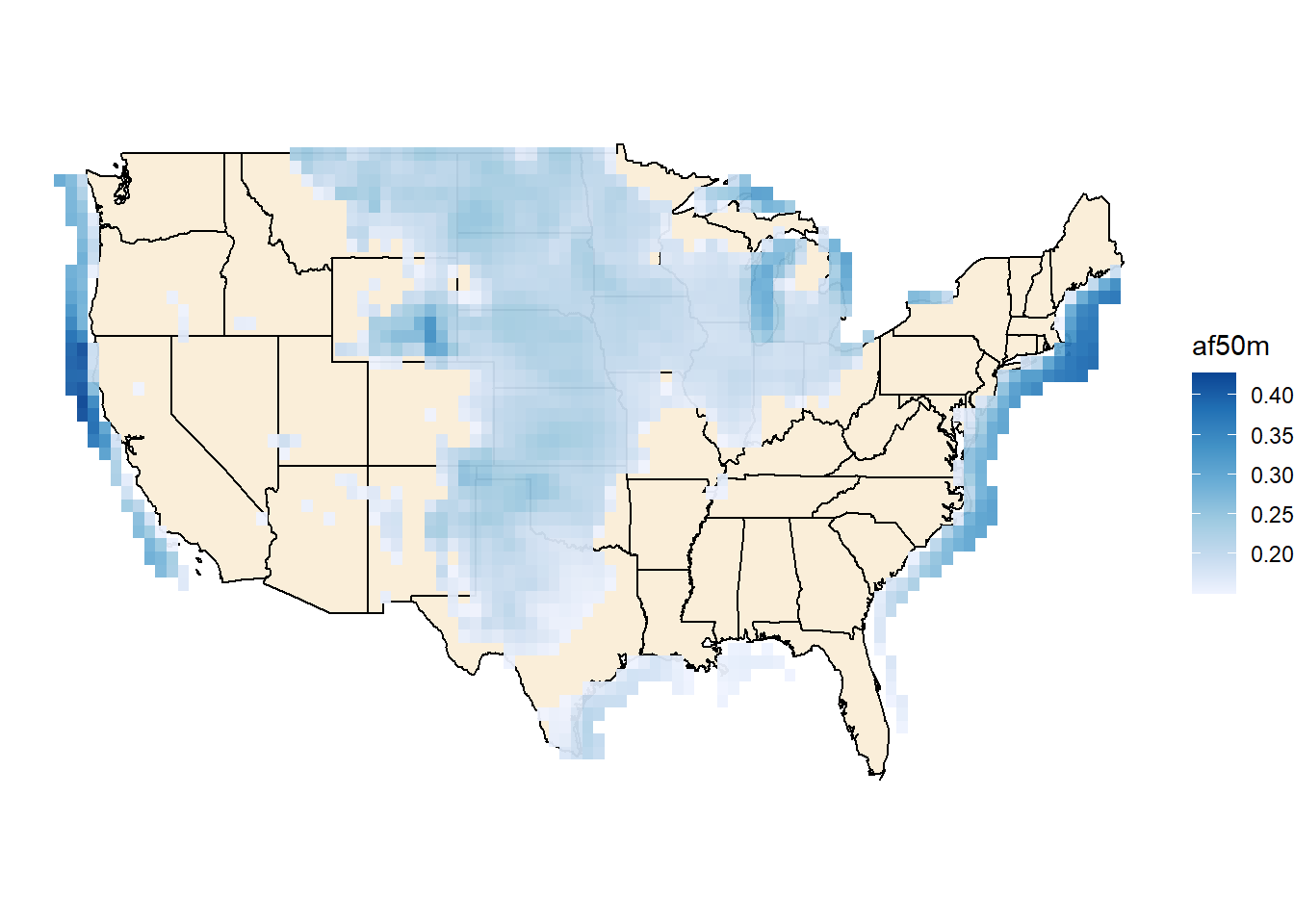
# filtered
ii <- ywnd$af50m >= .15; summary(ii)
##    Mode   FALSE    TRUE
## logical    1723    1300
ggywnd(ii)
## Warning: Raster pixels are placed at uneven horizontal intervals and will be
## shifted. Consider using geom_tile() instead.
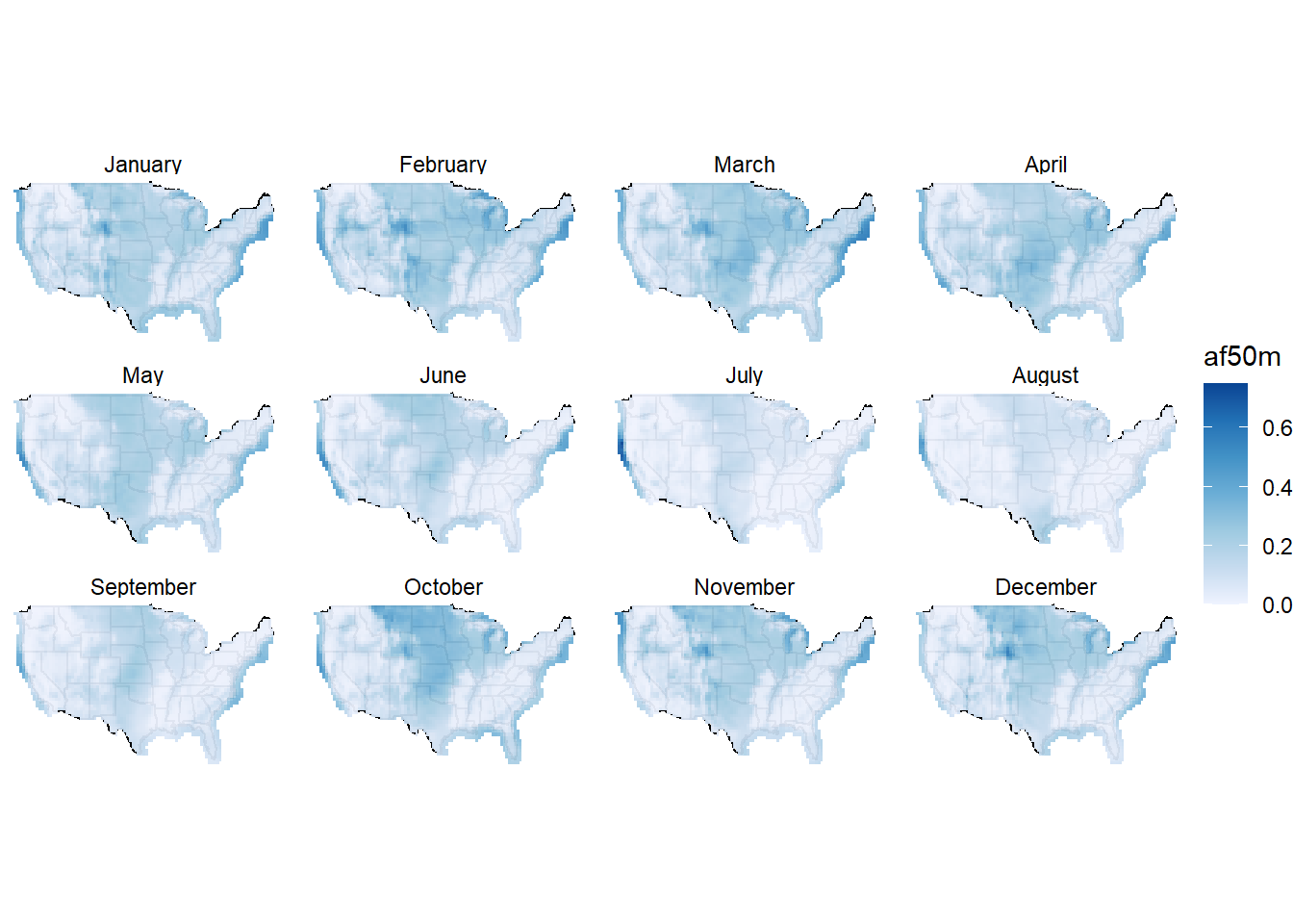
# Aggregation by months
mwnd <- group_by(gwnd, loc_id, lat, lon, region, month) %>%
summarise(af50m = sum(af50m/mdays)/24)
ggmwnd <- function(mm = rep(T, length(mwnd$loc_id))) {
ggplot(usa49r, aes(long,lat, group = group)) +
geom_polygon(colour = "black", fill = "wheat", alpha = .5) +
coord_fixed(1.45) +
theme_void() +
geom_raster(data = mwnd[mm,], aes(lon, lat, fill = af50m),
interpolate = F, inherit.aes = F, alpha = .95) +
scale_fill_distiller(palette = "Blues", direction = 1) + # , trans = "log10"
facet_wrap(.~month)
}
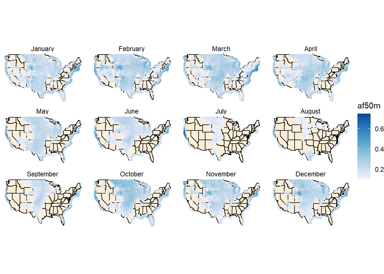
ggmwnd()
mm <- mwnd$af50m >= .1; summary(mm)
##    Mode   FALSE    TRUE
## logical   16570   19706
ggmwnd(mm)
# Averaging by annual potential
# `loc_id_??` is locations with the ranged potential
yy_20 <- ywnd$af50m >= .20; summary(yy_20); loc_id_20 <- ywnd$loc_id[yy_20]
##    Mode   FALSE    TRUE
## logical    2303     720
yy_15 <- ywnd$af50m >= .15 & ywnd$af50m < .20; summary(yy_15); loc_id_15 <- ywnd$loc_id[yy_15]
##    Mode   FALSE    TRUE
## logical    2443     580
yy_10 <- ywnd$af50m >= .10 & ywnd$af50m < .15; summary(yy_10); loc_id_10 <- ywnd$loc_id[yy_10]
##    Mode   FALSE    TRUE
## logical    2553     470
# Check for overlay
any(loc_id_20 %in% loc_id_15) | any(loc_id_10 %in% loc_id_20)
## [1] FALSE
# Assuming 4 megawatts per square kilometer (about 10 megawatts per square mile, NREL)
# for offshore: 3-5 megawatts (MW) per square kilometer
# Taking one grid cell is about ~50x60 km, or ~3000 sq.km,
# one grid cell can accomodate up to 12GW (3000 * 4 / 1e3) onshore or 9GW offshore.
# For simplicity let's assume up to 5GW can be used for both
# on- and off-shore wind power capacity per one cell of the grid.
# I.e. up to ~50% of therritory presumably might be used for wind energy
# from technical perspective. The number can be adjusted in constraints.
# hist(gwnd$af50m)
WINN_GW_max <- 5 # max GW Onshore per cell
WINF_GW_max <- 5 # max GW Offshore per cell
gwnd$max_GWh <- WINN_GW_max * gwnd$af50m # GWh per hour

# Onshore wind resource
# Filter and aggregate by regions locations
# with potential for locations with > 20% availability factor
ii <- (gwnd$loc_id %in% loc_id_20) & gwnd$US_10km_buffer
summary(ii)
##     Mode    FALSE     TRUE
##  logical 21707280  4774200
wnd_af20 <- group_by(gwnd[ii,], datetime, region) %>%
  summarise(max_GWh = sum(max_GWh, na.rm = T),
            af50m = mean(af50m))
wnd_af20
## # A tibble: 210,240 x 4
## # Groups:   datetime [8,760]
##    datetime            region max_GWh  af50m
##    <dttm>              <chr>    <dbl>  <dbl>
##  1 2017-01-01 00:30:00 CA        2.7  0.54
##  2 2017-01-01 00:30:00 CO        9.74 0.244
##  3 2017-01-01 00:30:00 DE        5    1
##  4 2017-01-01 00:30:00 IA       41.6  0.308
##  5 2017-01-01 00:30:00 IL        0.04 0.004
##  6 2017-01-01 00:30:00 KS       24.7  0.0771
##  7 2017-01-01 00:30:00 MA        9.48 0.948
##  8 2017-01-01 00:30:00 MD        3.1  0.62
##  9 2017-01-01 00:30:00 MI       25.1  0.295
## 10 2017-01-01 00:30:00 MN       78.7  0.375
## # ... with 210,230 more rows
sum(wnd_af20$max_GWh)/1e3 # Total estimated onshore potential
## [1] 5288.6
unique(wnd_af20$region) # regions with onshore wind potential
##  [1] "CA" "CO" "DE" "IA" "IL" "KS" "MA" "MD" "MI" "MN" "MT" "NC" "ND" "NE" "NJ"
## [16] "NM" "NY" "OH" "OK" "SD" "TX" "VA" "WI" "WY"
wnd_GW_max_reg <- group_by(gwnd[ii,], region, loc_id) %>%
  summarise(max_GWh = WINN_GW_max * sum(af50m),
            af50m = mean(af50m)) %>%
  ungroup() %>% group_by(region) %>%
  summarise(max_GW = WINN_GW_max * n(),
            max_GWh = sum(max_GWh))
sum(wnd_GW_max_reg$max_GWh/1e3); sum(wnd_af20$max_GWh)/1e3 # check
## [1] 5288.6
## [1] 5288.6
# Offshore wind resource
ii <- (gwnd$loc_id %in% loc_id_20) & gwnd$offshore
summary(ii)
##     Mode    FALSE     TRUE
##  logical 24948480  1533000
wndf_af20 <- group_by(gwnd[ii,], datetime, region) %>%
  summarise(max_GWh = sum(max_GWh, na.rm = T),
            af50m = mean(af50m))
wndf_af20
## # A tibble: 166,440 x 4
## # Groups:   datetime [8,760]
##    datetime            region max_GWh af50m
##    <dttm>              <chr>    <dbl> <dbl>
##  1 2017-01-01 00:30:00 CA      76.0   0.460
##  2 2017-01-01 00:30:00 DE       5     1
##  3 2017-01-01 00:30:00 IL       0.265 0.053
##  4 2017-01-01 00:30:00 MA      72.9   0.972
##  5 2017-01-01 00:30:00 MD      10     1
##  6 2017-01-01 00:30:00 ME      47.8   0.956
##  7 2017-01-01 00:30:00 MI      55.6   0.463
##  8 2017-01-01 00:30:00 MN       5     1
##  9 2017-01-01 00:30:00 NC      59.4   0.517
## 10 2017-01-01 00:30:00 NJ      29.1   0.972
## # ... with 166,430 more rows
sum(wndf_af20$max_GWh)/1e3 # Total offshore wind potential
## [1] 2250.915
unique(wndf_af20$region) # regions with offshore wind potential
##  [1] "CA" "DE" "IL" "MA" "MD" "ME" "MI" "MN" "NC" "NJ" "NY" "OH" "OR" "RI" "SC"
## [16] "TX" "VA" "WA" "WI"
wndf_GW_max_reg <- group_by(gwnd[ii,], region, loc_id) %>%
  summarise(af50m = mean(af50m),
            max_GWh = sum(af50m)) %>%
  ungroup() %>% group_by(region) %>%
  summarise(max_GW = 5 * n(),
            max_GWh = sum(af50m))
sum(wndf_af20$max_GWh)/1e3; sum(wndf_af20$max_GWh)/1e3 # check
## [1] 2250.915
## [1] 2250.915
Weather classes in the model
Weather classes (in the energyRt package) are used to store/add weather factors to the model data.
code
# Solar AF
# dim(dhsol)
# head(dhsol)
ii <- rep(T, dim(dhsol)[1]) # filter if needed

SOLAR_AF <- newWeather("SOLAR_AF",
                        description = "Ground level insolation AF",
                        # unit = "kWh/kWh_max",
                        slice = "HOUR",
                        weather = data.frame(
                          region = as.character(dhsol$region[ii]),
                          # year = 2018,
                          slice = dhsol$slice[ii],
                          wval = dhsol$WF[ii]
                        ))

head(SOLAR_AF@weather)
##   region year    slice wval
## 1     AL   NA d001_h00    0
## 2     AL   NA d001_h01    0
## 3     AL   NA d001_h02    0
## 4     AL   NA d001_h03    0
## 5     AL   NA d001_h04    0
## 6     AL   NA d001_h05    0
dim(SOLAR_AF@weather)[1] / 49 / 365 / 24 # Check: must be == 1
## [1] 1
# Wind AF (onshore)
wnd_af20$slice <- datetime2tsdh(wnd_af20$datetime)
wnd_af20
## # A tibble: 210,240 x 5
## # Groups:   datetime [8,760]
##    datetime            region max_GWh  af50m slice
##    <dttm>              <chr>    <dbl>  <dbl> <chr>
##  1 2017-01-01 00:30:00 CA        2.7  0.54   d001_h00
##  2 2017-01-01 00:30:00 CO        9.74 0.244  d001_h00
##  3 2017-01-01 00:30:00 DE        5    1      d001_h00
##  4 2017-01-01 00:30:00 IA       41.6  0.308  d001_h00
##  5 2017-01-01 00:30:00 IL        0.04 0.004  d001_h00
##  6 2017-01-01 00:30:00 KS       24.7  0.0771 d001_h00
##  7 2017-01-01 00:30:00 MA        9.48 0.948  d001_h00
##  8 2017-01-01 00:30:00 MD        3.1  0.62   d001_h00
##  9 2017-01-01 00:30:00 MI       25.1  0.295  d001_h00
## 10 2017-01-01 00:30:00 MN       78.7  0.375  d001_h00
## # ... with 210,230 more rows
dim(wnd_af20)[1] / 365/24 # number of regions with the onshore potential
## [1] 24
ii <- rep(T, dim(wnd_af20)[1]) #
summary(wnd_af20$af50m)
##    Min. 1st Qu.  Median    Mean 3rd Qu.    Max.
##  0.0000  0.0494  0.1493  0.2253  0.3231  1.0000
# wnd_af20$region <- as.character(wnd_af20$region)
WINON20_AF <- newWeather("WINON20_AF",
                        description = "Onshore wind potential af20",
                        region = unique(wnd_af20$region[ii]),
                        # unit = "kWh/kWh_max",
                        slice = "HOUR",
                        weather = data.frame(
                          region = as.character(wnd_af20$region[ii]),
                          # year = 2010,
                          slice = wnd_af20$slice[ii],
                          wval = wnd_af20$af50m[ii]
                        ))
head(WINON20_AF@weather)
##   region year    slice       wval
## 1     CA   NA d001_h00 0.54000000
## 2     CO   NA d001_h00 0.24350000
## 3     DE   NA d001_h00 1.00000000
## 4     IA   NA d001_h00 0.30848148
## 5     IL   NA d001_h00 0.00400000
## 6     KS   NA d001_h00 0.07714063
dim(WINON20_AF@weather)[1] / 365 / 24 # Check - number of regions with the data
## [1] 24
# Wind AF (offshore)
wndf_af20$slice <- datetime2tsdh(wndf_af20$datetime)
wndf_af20
## # A tibble: 166,440 x 5
## # Groups:   datetime [8,760]
##    datetime            region max_GWh af50m slice
##    <dttm>              <chr>    <dbl> <dbl> <chr>
##  1 2017-01-01 00:30:00 CA      76.0   0.460 d001_h00
##  2 2017-01-01 00:30:00 DE       5     1     d001_h00
##  3 2017-01-01 00:30:00 IL       0.265 0.053 d001_h00
##  4 2017-01-01 00:30:00 MA      72.9   0.972 d001_h00
##  5 2017-01-01 00:30:00 MD      10     1     d001_h00
##  6 2017-01-01 00:30:00 ME      47.8   0.956 d001_h00
##  7 2017-01-01 00:30:00 MI      55.6   0.463 d001_h00
##  8 2017-01-01 00:30:00 MN       5     1     d001_h00
##  9 2017-01-01 00:30:00 NC      59.4   0.517 d001_h00
## 10 2017-01-01 00:30:00 NJ      29.1   0.972 d001_h00
## # ... with 166,430 more rows
dim(wndf_af20)[1] / 365/24
## [1] 19
ii <- rep(T, dim(wndf_af20)[1]) #
summary(wndf_af20$af50m)
##    Min. 1st Qu.  Median    Mean 3rd Qu.    Max.
## 0.00000 0.04948 0.18450 0.27774 0.42129 1.00000
wndf_af20$region <- as.character(wndf_af20$region)
WINOF20_AF <- newWeather("WINOF20_AF",
                        description = "Offshore wind potential af20",
                        # unit = "kWh/kWh_max",
                        region = unique(wndf_af20$region),
                        slice = "HOUR",
                        weather = data.frame(
                          region = as.character(wndf_af20$region[ii]),
                          # year = 2010,
                          slice = wndf_af20$slice[ii],
                          wval = wndf_af20$af50m[ii]
                        ))
head(WINOF20_AF@weather)
##   region year    slice      wval
## 1     CA   NA d001_h00 0.4603636
## 2     DE   NA d001_h00 1.0000000
## 3     IL   NA d001_h00 0.0530000
## 4     MA   NA d001_h00 0.9717333
## 5     MD   NA d001_h00 1.0000000
## 6     ME   NA d001_h00 0.9564000
dim(WINOF20_AF@weather)[1] / 365 / 24
## [1] 19
Supply
Declaration of resources (upstream technologies) in the model.
Here we use only solar and wind energy.
code
RES_SOL <- newSupply(
  name = "RES_SOL",
  description = "Terrestrial solar radiation - maximum potential",
  commodity = "SOL",
  unit = "GWh",
# Weather factors could be used to regulate hourly supply of the resources.
# Though to reduce the model dimension, it is enough to use
# weather factors in technologies.
  # weather = data.frame(
  #   weather = c("SOLAR_AF"),
  #   wava.up =  c(1)
  #   ),
  # availability = list(
  #   # region = dh$region,
  #   # slice = dh$slice365,
  #   ava.up = 1e10 # Max available resource in hour, i.e. no limit by now
  # ),
  slice = "ANNUAL"
)

RES_WIN <- newSupply(
  name = "RES_WIN",
  description = "Onshore wind - maximum potential",
  commodity = "WIN",
  region = unique(wnd_af20$region),
  unit = "GWh",
  # weather = data.frame(
  #   weather = c("SOLAR_AF"),
  #   wava.up =  c(1)
  #   ),
#   availability = list(
#     region = wnd_af20$region,
#     slice = wnd_af20$slice,
# # here is an alternative (equivalent) way to use weather factors in supply
#     ava.up = wnd_af20$max_GWh # Max available resource in hour
#   ),
  slice = "ANNUAL"
)

RES_WFF <- newSupply(
  name = "RES_WFF",
  description = "Offshore wind - maximum potential",
  commodity = "WFF",
  region = unique(wndf_af20$region),
  unit = "GWh",
  # weather = data.frame(
  #   weather = c("SOLAR_AF"),
  #   wava.up =  c(1)
  #   ),
  # availability = list(
  #   region = wndf_af20$region,
  #   slice = wndf_af20$slice,
  #   ava.up = wndf_af20$max_GWh # Max available resource in hour
  # ),
  slice = "ANNUAL"
)

SUP_BIO <- newSupply(
  name = "SUP_BIO",
  description = "Biomass resource, annual",
  commodity = "BIO",
  unit = "GWh",
  availability = data.frame(
    cost = convert("USD/kWh", "MUSD/GWh", .05) # arbitrary, assuming expensive
  ),
  slice = "ANNUAL"
)
Power generating technologies
code
ESOL <- newTechnology(
  name = "ESOL",
  description = "Utility Scale Solar PV",
  # region = "AZ",
  input = list(
    comm = "SOL",
    unit = "GWh"
  ),
  output = list(
    comm = "ELC",
    unit = "GWh"
  ),
  cap2act = 365*24,
  af = list(
    af.fx = 1 # forcing output when resource is available
  ),
  weather = list(
    weather = c("SOLAR_AF"),
    waf.fx = 1 # weather factor (multiplier) will be applied to af.fx
  ),
  fixom = list(
    fixom = 10 # assumed, 1% of investment costs a year
  ),
  invcost = list(
    # Assuming 1$/Watt
    # https://www.nrel.gov/news/press/2017/nrel-report-utility-scale-solar-pv-system-cost-fell-last-year.html
    invcost = 1000 # convert("USD/W", "MUSD/GW", 1)
  ),
  start = list(
    start = 2018
  ),
  olife = list(
    olife = 25
  )
)
draw(ESOL)

EWIN <- newTechnology(
  name = "EWIN",
  description = "Onshore wind farm",
   WINON20_AF@region, # Limiting to regions with available resource
  input = list(
    comm = "WIN",
    unit = "GWh"
  ),
  output = list(
    comm = "ELC",
    unit = "GWh"
  ),
  cap2act = 365*24,
  af = list(
    af.fx = 1 # forcing output when resource is available
  ),
  weather = list(
    weather = c("WINON20_AF"),
    waf.fx = c(1)
    # waf.up = c(1) #
  ),
  fixom = list(
    fixom = 15 # Assumed, 1% a year
  ),
  invcost = list(
    # Assuming 1.5$/Watt
    # https://www.irena.org/-/media/Files/IRENA/Agency/Publication/2018/Jan/IRENA_2017_Power_Costs_2018.pdf
    invcost = 1500 #
  ),
  start = list(
    start = 2018
  ),
  olife = list(
    olife = 25
  )
)
draw(EWIN)

EWFF <- newTechnology(
  name = "EWFF",
  description = "Offshore wind farm",
  region = WINOF20_AF@region, # Limiting to regions with available resource
  input = list(
    comm = "WFF",
    unit = "GWh"
  ),
  output = list(
    comm = "ELC",
    unit = "GWh"
  ),
  cap2act = 365*24,
  af = list(
    af.fx = 1 # forcing output when resource is available
  ),
  weather = list(
    weather = c("WINOF20_AF"),
    waf.up = c(1) #
  ),
  fixom = list(
    fixom = 45 # Assumed, 1% a year
  ),
  invcost = list(
    # Assuming 3-4.5$/Watt
    # https://www.irena.org/-/media/Files/IRENA/Agency/Publication/2018/Jan/IRENA_2017_Power_Costs_2018.pdf
    # https://www.energy.gov/sites/prod/files/2019/08/f65/2018%20Offshore%20Wind%20Market%20Report.pdf
    invcost = 3500 # convert("USD/W", "MUSD/GW", 1)
  ),
  start = list(
    start = 2018
  ),
  olife = list(
    olife = 25
  )
)
draw(EWFF)

CSOL_UP <- newConstraintS(
  name = "CSOL_UP",
  eq = "<=",
  type = "capacity",
  for.each = data.frame(
    year = USENSYS$modelYear,
    tech = "ESOL",
    region = as.character(PV_GW_max_reg$region)),
  rhs = data.frame(
    # year = USENSYS$modelYear,
    # tech = "ESOL",
    region = as.character(PV_GW_max_reg$region),
    rhs = PV_GW_max_reg$GW_up
  )) # limit on solar capacity (resource)

CWIN_UP <- newConstraintS(
  name = "CWIN_UP",
  eq = "<=",
  type = "capacity",
  for.each = data.frame(
    year = USENSYS$modelYear,
    tech = "EWIN",
    region = wnd_GW_max_reg$region),
  rhs = data.frame(
    region = wnd_GW_max_reg$region,
    rhs = wnd_GW_max_reg$max_GW)) # limit on onshore wind capacity (resource)

CWFF_UP <- newConstraintS(
  name = "CWFF_UP",
  eq = "<=",
  type = "capacity",
  for.each = list(
    year = USENSYS$modelYear,
    tech = "EWFF",
    region = wndf_GW_max_reg$region),
  rhs = data.frame(
    region = wndf_GW_max_reg$region,
    rhs = wndf_GW_max_reg$max_GW)) # limit on onshore wind capacity (resource)
Thermal backup
Generic thermal technology as a back-up capacity to cover gaps between renewables generation and consumption, for example, biomass-, biogas-to-power or conventional natural gas turbines. The idea of adding the technology to the optimization, is to identify potential substitution between storage, grid, and back-up capacity. To avoid use of the technology for base load generation, we assume high costs and upper bounds on the availability factor.
code
BIO <- newCommodity('BIO', slice = "ANNUAL")

EBIO <- newTechnology(
  name = "EBIO",
  description = "Thermal backup",
  input = list(
    comm = "BIO",
    unit = "GWh"
  ),
  output = list(
    comm = "ELC",
    unit = "GWh"
  ),
  cap2act = 365*24,
  afs = list(
    slice = "ANNUAL",
    # afs.up = .1 # up tp 10% capacity usitilization through the year
    afs.up = .4 # up to 40% capacity usitilization through the year
  ),
  ceff = list(
    comm = "BIO",
    cinp2use = .4
  ),
  invcost = list(
    invcost = 2400 #
  ),
  # fixom = list(
  #   fixom = 20 # Assumed, 2% a year
  # ),
  # see the fuel cost
  # varom = list(
  #   varom = convert("cents/kWh", "MUSD/GWh", 5) # assuming expensive operation
  # ),
  olife = list(
    olife = 20
  ),
  slice = "HOUR"
)
draw(EBIO)

# (1200/20 + 20/20 + 0.1*365*24*.05/.4)/ (365*24*.1)
Storage technologies
code
# STGBTR Hourly ####
# See IRENA 2030 (from 77 to 574, p.77)
# NREL, 4-hours battery storage, grid-connected
STGBTR <- newStorage(
  name = 'STGBTR',
  commodity = 'ELC',
  description = "Generic grid-integrated storage, 1 hour plus",
  cap2stg = 1, # in kWh or 1-hour storage
  olife = list(olife = 20),
  invcost = list(
    invcost = convert("USD/kWh", "MUSD/GWh", 300)
    #
    ),
  seff = data.frame(
    inpeff = 0.8, # assumed efficiency of charging
    stgeff = 0.9 # assumed efficiency of storing energy (annual)
    # outeff = 1 # discharge efficiency
    )
)

# STGBTR1 <- newStorage(
#   name = 'STGBTR',
#   commodity = 'ELC',
#   description = "Generic grid-integrated intraday storage (battery)",
#   cap2stg = 4, # 4-hours battery
#   olife = list(olife = 20),
#   invcost = list(
#     # See IRENA 2030 (from 77 to 574, p.77)
#     # invcost = convert("USD/kWh", "MUSD/GWh", 200)
#     invcost = convert("USD/kW", "MUSD/GW", 300 * 4) # 1200 USD/kW for 4-hours battery
#     ),
#   seff = data.frame(
#     inpeff = 0.8, # assumed efficiency of charging
#     stgeff = 0.9, # assumed efficiency of storing energy (annual)
#     cinp.up = 24*365 / 4, # 4-hours charging
#     cout.up = 24*365 / 4 # 4-hours storage (discharging, i.e. GW capacity)
#     # outeff = 1 # discharge efficiency
#     )
# )
#
#
# # STGP2P Daily - within 365 days ####
STGP2P <- newStorage(
  name = 'STGP2P',
  commodity = 'ELC',
  description = "Power-to-power type of technology",
  cap2stg = 100, # if in PJ, convert("GWh", "PJ"),
  olife = list(
    olife = 25),
  invcost = 100, # USD/kWh, assumption
  seff = data.frame(
    inpeff = 0.8, # power to H2 efficiency
    cinp.up = 24*365, # speed of P2X conversion for 1GW of storage
    cout.up = 24*365,  # speed of X2P conversion for 1GW of storage
    outeff = 0.625 # H2 to power efficiency
    # # stgeff = .9
    # cinp.up = 24*365,
    # cout.up = 24*365
    ),
  varom = list(
    # Assuming high operational costs, adding ~ 5 cents/kWh
    inpcost = convert("USD/kWh", "MUSD/GWh", .05)
    )
)
Interregional UHV electrical grid
code
# Propose trade matrix between regions
{
if (F) {
  # Load trade matrix from your file
  trd_xl <- readxl::read_excel("data/trade_matrix01.xlsx",
                               range = "A1:AX50")

  trd_nbr <- as.matrix(trd_xl[,-1])
  trd_nbr[lower.tri(trd_nbr)] <- NA
  rownames(trd_nbr) <- trd_xl$region
} else {
  # Or create trade matrix for all neighbour regions
  trd_nbr <- matrix(rep(NA, nreg_in_gis*nreg_in_gis),
                    nrow = nreg_in_gis,
                    dimnames = list(reg_names_in_gis, reg_names_in_gis))
  head(trd_nbr)

  for (i in 1:length(reg_names)) {
    trd_nbr[i, nbr[[i]]] <- 1
    trd_nbr[nbr[[i]], i] <- 1
  }
  dim(trd_nbr)
  summary(!is.na(c(trd_nbr)))
  ii <- reg_names_in_gis %in% reg_names
  trd_nbr <- trd_nbr[ii, ii]
  dim(trd_nbr)
  # For bidirectional trade, keep only one direction
  trd_nbr[lower.tri(trd_nbr)] <- NA
  summary(!is.na(c(trd_nbr)))
}
head(trd_nbr)
# write.csv(trd_nbr, file = "data/trade_matrix.csv")
trd_nbr[trd_nbr == 0] <- NA

# Convert the matrix to data.frame (table) format
trd_dt <- as.data.frame.table(trd_nbr, stringsAsFactors = F)
trd_dt <- trd_dt[!is.na(trd_dt$Freq),]
head(trd_dt)
dim(trd_dt)
trd_dt <- dplyr::distinct(trd_dt)
dim(trd_dt)
names(trd_dt) <- c("src", "dst", "trade")
trd_dt$trade <- with(trd_dt, paste0("TRBD_UHV_", src, "_", dst))
head(trd_dt)

# Map region flows
trd_map <- left_join(trd_dt, reg_centers[,1:3], by = c("src" = "region"))
trd_map <- left_join(trd_map, reg_centers[,1:3], by = c("dst" = "region"))
trd_map <- trd_map %>%
  rename(xsrc = x.x, ysrc = y.x,
         xdst = x.y, ydst = y.y)
trd_map <- as_tibble(trd_map)

# Filter excessive connections
dim(trd_dt); dim(trd_map)
drop_route <- function(reg1, reg2) {
  (trd_dt$src == reg1 & trd_dt$dst == reg2) | (trd_dt$src == reg2 & trd_dt$dst == reg1)
}
# trd_dt[ii & grepl("TJ", trd_dt$trade),]
ii <- rep(TRUE, length(trd_dt$src))
ii <- ii & !drop_route("AL", "FL")
ii <- ii & !drop_route("GA", "NC")
ii <- ii & !drop_route("CT", "RI")
ii <- ii & !drop_route("VT", "MA")
ii <- ii & !drop_route("NY", "MA")
ii <- ii & !drop_route("PA", "DE")
ii <- ii & !drop_route("UT", "NM")
ii <- ii & !drop_route("VA", "DC")
ii <- ii & !drop_route("AL", "TN")
if (F) {
  # Drop unused routes (scen_REN5)
  # names(TRBD_UHV_NEI@data)[!(names(TRBD_UHV_NEI@data) %in% vTradeCap$trade[!is.na(vTradeCap$GW)])]
  #  [1] "TRBD_UHV_SD_MN" "TRBD_UHV_WI_IA" "TRBD_UHV_NY_NJ"
  #  [4] "TRBD_UHV_OR_NV" "TRBD_UHV_ID_UT" "TRBD_UHV_WV_MD"
  #  [7] "TRBD_UHV_KY_VA" "TRBD_UHV_NE_MO" "TRBD_UHV_CO_AZ"
  # [10] "TRBD_UHV_OK_NM" "TRBD_UHV_TX_AR"
  ii <- ii & !drop_route("SD", "MN")
  ii <- ii & !drop_route("WI", "IA")
  ii <- ii & !drop_route("NY", "NJ")
  ii <- ii & !drop_route("OR", "NV")
  ii <- ii & !drop_route("ID", "UT")
  ii <- ii & !drop_route("WV", "MD")
  ii <- ii & !drop_route("KY", "VA")
  # ii <- ii & !drop_route("NE", "MO")
  ii <- ii & !drop_route("CO", "AZ")
  ii <- ii & !drop_route("OK", "NM")
  ii <- ii & !drop_route("TX", "AR")
  # Drop more (after optimization check)
  ii <- ii & !drop_route("VA", "TN")
  # ii <- ii & !drop_route("MO", "TN")
  ii <- ii & !drop_route("NC", "TN")
  ii <- ii & !drop_route("KY", "MO")
  ii <- ii & !drop_route("KY", "WV")
  ii <- ii & !drop_route("NV", "AZ")
}
length(trd_dt$src[ii])

library(ggrepel)
trd_flows_map <-
ggplot(data = usa49r) +
  geom_polygon(aes(x = long, y = lat, group = group), fill = "wheat",
               colour = "white", alpha = 1, size = .5) + # aes fill = id,
  coord_fixed(1.3) +
  guides(fill=FALSE) +  # do this to leave off the color legend
  theme_void() + labs(title = "Interregional electricity trade routes (long distance grid), open for investment")  +
  theme(plot.title = element_text(hjust = 0.5),
        plot.subtitle = element_text(hjust = 0.5)) +
  geom_segment(aes(x=xsrc, y=ysrc, xend=xdst, yend=ydst),
               data = trd_map[ii,], inherit.aes = FALSE, size = 3,
               alpha = 1, colour = "grey", lineend = "round", show.legend = T) +
  geom_point(data = reg_centers, aes(x, y), colour = "white") +
  geom_segment(aes(x=xsrc, y=ysrc, xend=xdst, yend=ydst),
               data = trd_map[ii,], inherit.aes = FALSE, size = .1,
           # arrow = arrow(type = "closed", angle = 15,
           #               length = unit(0.15, "inches")),
           colour = "white", alpha = 1,
           lineend = "butt", linejoin = "mitre", show.legend = T) + # , name = "Trade, PJ"
  geom_text_repel(aes(x, y, label = region), data = reg_centers)
trd_flows_map
trd_map <- trd_map[ii,]; rownames(trd_map) <- NULL
trd_dt <- trd_dt[ii,]; rownames(trd_dt) <- NULL
# ggsave("fig/trd_flows_map.pdf", trd_flows_map, device = "pdf")
}
# Calculate distance between regions centers:
labpt <- getCenters(usa49reg)
# rownames(labpt) <- labpt[,"region"]

# Estimate grid length, losses, costs
trd_dt$distance_km <- 0.
for (i in 1:dim(trd_dt)[1]) {
  rg_dst <- trd_dt$dst[i]
  rg_src <- trd_dt$src[i]
  ii <- labpt$region == rg_dst
  lab_dst <- c(labpt$x[ii], labpt$y[ii])
  ii <- labpt$region == rg_src
  lab_src <- c(labpt$x[ii], labpt$y[ii])
  trd_dt$distance_km[i] <- raster::pointDistance(
    lab_src, lab_dst, T)/1e3
}

# Assume 15% longer distance due to a landscape
trd_dt$distance_km <- 1.15 * trd_dt$distance_km
# Assume losses 2% per 1000 km
# trd_dt$losses <- round(trd_dt$distance_km / 1e3 * 0.02, 4)
# Assume losses 1% per 1000 km (UHVDC)
trd_dt$losses <- round(trd_dt$distance_km / 1e3 * 0.01, 4)
trd_dt$teff <- 1 - trd_dt$losses
# The assumption is based on ABB's 4000-8000 MUSD per 12GW UHVDC, 2000km, 1-5% system losses
# i.e. ~$160-333 MUSD/1000km per 1GW of the total system
# assuming ~$200 MUSD/1000km per 1GW of power line,
# and $50 MUSD/GW for 1GW converter stations on each end
trd_dt$invcost <- round(trd_dt$distance_km / 1e3 * 200) # MUSD/GW of 1000km UHVDC
trd_dt$invcost <- round(trd_dt$invcost * 1.5) # Adding land costs (50%, an assumption)
trd_dt <- as_tibble(trd_dt)

# Define trade object for every route,
# store in a repository object
TRBD_UHV_NEI <- newRepository(name = "TRBD_UHV_NEI")
for (i in 1:dim(trd_dt)[1]) {
  src <- trd_dt$src[i]
  dst <- trd_dt$dst[i]
  trd_nm <- paste0("TRBD_UHV_", src, "_", dst)  # Trade object name
  cmd_nm <- "UHV"
  # Trade class for every route
  trd <- newTrade(trd_nm,
                  commodity = cmd_nm,
                  # source = c(src, dst),
                  # destination = c(src, dst),
                  routes = list(
                    src = c(src, dst),
                    dst = c(dst, src)
                  ),
                  trade = data.frame(
                    src = c(src, dst),
                    dst = c(dst, src),
                    # Maximum capacity per route in GW
                    # ava.up = convert("GWh", "GWh", 60), (!!! bug)
                    teff = trd_dt$teff[i] # trade losses
                    # cost = trd_dt$cost[i]  # trade costs
                    # markup = trd_dt$cost[i] # and/or markup
                    ),
                  #!!! New stuff - testing
                  capacityVariable = TRUE, # The trade route has capacity (not just flow) and can be endogenous
                  # bidirectional = TRUE, #
                  invcost = data.frame(
                    # src = src,
                    # dst = dst,
                    # year = 2010,
                    region = c(dst, src),
                    # invcost = trd_dt$distance_km[i] / 1e3 * 250 / 2 #
                    invcost = trd_dt$invcost[i] / 2
                  ),
                  # olife = data.frame(
                  olife = 80,
                  # ),
                  cap2act = convert("GWh", "GWh", 24*365)
                  )

  TRBD_UHV_NEI <- add(TRBD_UHV_NEI, trd)
}
rm(trd)
length(TRBD_UHV_NEI@data)
## [1] 100
names(TRBD_UHV_NEI@data)
##   [1] "TRBD_UHV_MT_ND" "TRBD_UHV_MT_SD" "TRBD_UHV_ND_SD" "TRBD_UHV_MT_WY"
##   [5] "TRBD_UHV_SD_WY" "TRBD_UHV_WA_ID" "TRBD_UHV_MT_ID" "TRBD_UHV_WY_ID"
##   [9] "TRBD_UHV_ND_MN" "TRBD_UHV_SD_MN" "TRBD_UHV_WI_MN" "TRBD_UHV_WA_OR"
##  [13] "TRBD_UHV_ID_OR" "TRBD_UHV_ME_NH" "TRBD_UHV_VT_NH" "TRBD_UHV_SD_IA"
##  [17] "TRBD_UHV_WI_IA" "TRBD_UHV_MN_IA" "TRBD_UHV_NH_MA" "TRBD_UHV_SD_NE"
##  [21] "TRBD_UHV_WY_NE" "TRBD_UHV_IA_NE" "TRBD_UHV_VT_NY" "TRBD_UHV_NY_PA"
##  [25] "TRBD_UHV_MA_CT" "TRBD_UHV_NY_CT" "TRBD_UHV_MA_RI" "TRBD_UHV_NY_NJ"
##  [29] "TRBD_UHV_PA_NJ" "TRBD_UHV_ID_NV" "TRBD_UHV_OR_NV" "TRBD_UHV_WY_UT"
##  [33] "TRBD_UHV_ID_UT" "TRBD_UHV_NV_UT" "TRBD_UHV_OR_CA" "TRBD_UHV_NV_CA"
##  [37] "TRBD_UHV_PA_OH" "TRBD_UHV_IN_OH" "TRBD_UHV_WI_IL" "TRBD_UHV_IA_IL"
##  [41] "TRBD_UHV_IN_IL" "TRBD_UHV_NJ_DE" "TRBD_UHV_PA_WV" "TRBD_UHV_OH_WV"
##  [45] "TRBD_UHV_PA_MD" "TRBD_UHV_DC_MD" "TRBD_UHV_DE_MD" "TRBD_UHV_WV_MD"
##  [49] "TRBD_UHV_WY_CO" "TRBD_UHV_NE_CO" "TRBD_UHV_UT_CO" "TRBD_UHV_IN_KY"
##  [53] "TRBD_UHV_OH_KY" "TRBD_UHV_IL_KY" "TRBD_UHV_WV_KY" "TRBD_UHV_NE_KS"
##  [57] "TRBD_UHV_CO_KS" "TRBD_UHV_WV_VA" "TRBD_UHV_MD_VA" "TRBD_UHV_KY_VA"
##  [61] "TRBD_UHV_IA_MO" "TRBD_UHV_NE_MO" "TRBD_UHV_IL_MO" "TRBD_UHV_KY_MO"
##  [65] "TRBD_UHV_KS_MO" "TRBD_UHV_NV_AZ" "TRBD_UHV_UT_AZ" "TRBD_UHV_CA_AZ"
##  [69] "TRBD_UHV_CO_AZ" "TRBD_UHV_CO_OK" "TRBD_UHV_KS_OK" "TRBD_UHV_MO_OK"
##  [73] "TRBD_UHV_VA_NC" "TRBD_UHV_KY_TN" "TRBD_UHV_VA_TN" "TRBD_UHV_MO_TN"
##  [77] "TRBD_UHV_NC_TN" "TRBD_UHV_OK_TX" "TRBD_UHV_CO_NM" "TRBD_UHV_AZ_NM"
##  [81] "TRBD_UHV_OK_NM" "TRBD_UHV_TX_NM" "TRBD_UHV_TN_MS" "TRBD_UHV_AL_MS"
##  [85] "TRBD_UHV_TN_GA" "TRBD_UHV_AL_GA" "TRBD_UHV_NC_SC" "TRBD_UHV_GA_SC"
##  [89] "TRBD_UHV_MO_AR" "TRBD_UHV_OK_AR" "TRBD_UHV_TN_AR" "TRBD_UHV_TX_AR"
##  [93] "TRBD_UHV_MS_AR" "TRBD_UHV_TX_LA" "TRBD_UHV_MS_LA" "TRBD_UHV_AR_LA"
##  [97] "TRBD_UHV_GA_FL" "TRBD_UHV_WI_MI" "TRBD_UHV_IN_MI" "TRBD_UHV_OH_MI"
TRBD_UHV_NEI@data[[1]]@invcost
##   region year invcost
## 1     ND   NA     120
## 2     MT   NA     120
mobj <- c(mobj, "trd_dt", "trd_map")
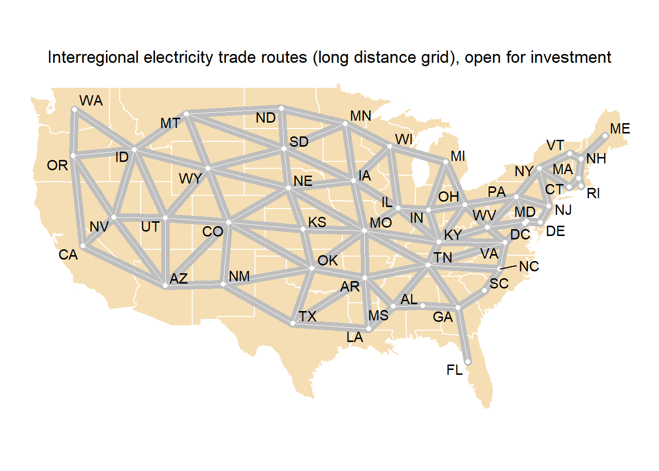
Figure 2: Endogenous trade routes (UHVDC lines)
Exogenous trade routes
code
TRFX_UHV_NEI <- newRepository("TRFX_UHV_NEI")
# emptrd <- newTrade("EmptyClassTrade")
for (i in 1:length(TRBD_UHV_NEI@data)) {
  route <- TRBD_UHV_NEI@data[[i]]
  # route@capacityVariable <- FALSE
  # route@invcost <- emptrd@invcost
  # route@olife <-  emptrd@olife
  # route@cap2act <-  emptrd@cap2act
  # route@trade$ava.up <- 60 # Assumption
  route@stock <- data.frame(year = 2018, stock = 60) # Assumption
  route@start <- 2100
  route@name <- sub("^TRBD", "TRFX", route@name)
  TRFX_UHV_NEI <- add(TRFX_UHV_NEI, route)
}

names(TRFX_UHV_NEI@data)
##   [1] "TRFX_UHV_MT_ND" "TRFX_UHV_MT_SD" "TRFX_UHV_ND_SD" "TRFX_UHV_MT_WY"
##   [5] "TRFX_UHV_SD_WY" "TRFX_UHV_WA_ID" "TRFX_UHV_MT_ID" "TRFX_UHV_WY_ID"
##   [9] "TRFX_UHV_ND_MN" "TRFX_UHV_SD_MN" "TRFX_UHV_WI_MN" "TRFX_UHV_WA_OR"
##  [13] "TRFX_UHV_ID_OR" "TRFX_UHV_ME_NH" "TRFX_UHV_VT_NH" "TRFX_UHV_SD_IA"
##  [17] "TRFX_UHV_WI_IA" "TRFX_UHV_MN_IA" "TRFX_UHV_NH_MA" "TRFX_UHV_SD_NE"
##  [21] "TRFX_UHV_WY_NE" "TRFX_UHV_IA_NE" "TRFX_UHV_VT_NY" "TRFX_UHV_NY_PA"
##  [25] "TRFX_UHV_MA_CT" "TRFX_UHV_NY_CT" "TRFX_UHV_MA_RI" "TRFX_UHV_NY_NJ"
##  [29] "TRFX_UHV_PA_NJ" "TRFX_UHV_ID_NV" "TRFX_UHV_OR_NV" "TRFX_UHV_WY_UT"
##  [33] "TRFX_UHV_ID_UT" "TRFX_UHV_NV_UT" "TRFX_UHV_OR_CA" "TRFX_UHV_NV_CA"
##  [37] "TRFX_UHV_PA_OH" "TRFX_UHV_IN_OH" "TRFX_UHV_WI_IL" "TRFX_UHV_IA_IL"
##  [41] "TRFX_UHV_IN_IL" "TRFX_UHV_NJ_DE" "TRFX_UHV_PA_WV" "TRFX_UHV_OH_WV"
##  [45] "TRFX_UHV_PA_MD" "TRFX_UHV_DC_MD" "TRFX_UHV_DE_MD" "TRFX_UHV_WV_MD"
##  [49] "TRFX_UHV_WY_CO" "TRFX_UHV_NE_CO" "TRFX_UHV_UT_CO" "TRFX_UHV_IN_KY"
##  [53] "TRFX_UHV_OH_KY" "TRFX_UHV_IL_KY" "TRFX_UHV_WV_KY" "TRFX_UHV_NE_KS"
##  [57] "TRFX_UHV_CO_KS" "TRFX_UHV_WV_VA" "TRFX_UHV_MD_VA" "TRFX_UHV_KY_VA"
##  [61] "TRFX_UHV_IA_MO" "TRFX_UHV_NE_MO" "TRFX_UHV_IL_MO" "TRFX_UHV_KY_MO"
##  [65] "TRFX_UHV_KS_MO" "TRFX_UHV_NV_AZ" "TRFX_UHV_UT_AZ" "TRFX_UHV_CA_AZ"
##  [69] "TRFX_UHV_CO_AZ" "TRFX_UHV_CO_OK" "TRFX_UHV_KS_OK" "TRFX_UHV_MO_OK"
##  [73] "TRFX_UHV_VA_NC" "TRFX_UHV_KY_TN" "TRFX_UHV_VA_TN" "TRFX_UHV_MO_TN"
##  [77] "TRFX_UHV_NC_TN" "TRFX_UHV_OK_TX" "TRFX_UHV_CO_NM" "TRFX_UHV_AZ_NM"
##  [81] "TRFX_UHV_OK_NM" "TRFX_UHV_TX_NM" "TRFX_UHV_TN_MS" "TRFX_UHV_AL_MS"
##  [85] "TRFX_UHV_TN_GA" "TRFX_UHV_AL_GA" "TRFX_UHV_NC_SC" "TRFX_UHV_GA_SC"
##  [89] "TRFX_UHV_MO_AR" "TRFX_UHV_OK_AR" "TRFX_UHV_TN_AR" "TRFX_UHV_TX_AR"
##  [93] "TRFX_UHV_MS_AR" "TRFX_UHV_TX_LA" "TRFX_UHV_MS_LA" "TRFX_UHV_AR_LA"
##  [97] "TRFX_UHV_GA_FL" "TRFX_UHV_WI_MI" "TRFX_UHV_IN_MI" "TRFX_UHV_OH_MI"
TRFX_UHV_NEI@data[[1]]
## An object of class "trade"
## Slot "name":
## [1] "TRFX_UHV_MT_ND"
##
## Slot "description":
## [1] ""
##
## Slot "commodity":
## [1] "UHV"
##
## Slot "routes":
##   src dst
## 1  MT  ND
## 2  ND  MT
##
## Slot "trade":
##   src dst year slice ava.up ava.fx ava.lo cost markup  teff
## 1  MT  ND   NA  <NA>     NA     NA     NA   NA     NA 0.992
## 2  ND  MT   NA  <NA>     NA     NA     NA   NA     NA 0.992
##
## Slot "aux":
## [1] acomm unit
## <0 rows> (or 0-length row.names)
##
## Slot "aeff":
## [1] acomm     src       dst       year      slice     csrc2aout csrc2ainp
## [8] cdst2aout cdst2ainp
## <0 rows> (or 0-length row.names)
##
## Slot "invcost":
##   region year invcost
## 1     ND   NA     120
## 2     MT   NA     120
##
## Slot "olife":
## [1] 80
##
## Slot "start":
## [1] 2100
##
## Slot "end":
## [1] Inf
##
## Slot "stock":
##   year stock
## 1 2018    60
##
## Slot "capacityVariable":
## [1] TRUE
##
## Slot "GIS":
## NULL
##
## Slot "cap2act":
## [1] 8760
##
## Slot "misc":
## list()
##
## Slot ".S3Class":
## [1] "trade"
# Dropping converter stations
TRFX_ELC_NEI <- newRepository("TRFX_ELC_NEI")
# emptrd <- newTrade("EmptyClassTrade")
for (i in 1:length(TRFX_UHV_NEI@data)) {
  route <- TRFX_UHV_NEI@data[[i]]
  route@commodity <- "ELC"
  # route@trade$ava.up <- 60 # Assumption
  route@name <- sub("_UHV_", "_ELC_", route@name)
  TRFX_ELC_NEI <- add(TRFX_ELC_NEI, route)
}

names(TRFX_ELC_NEI@data)
##   [1] "TRFX_ELC_MT_ND" "TRFX_ELC_MT_SD" "TRFX_ELC_ND_SD" "TRFX_ELC_MT_WY"
##   [5] "TRFX_ELC_SD_WY" "TRFX_ELC_WA_ID" "TRFX_ELC_MT_ID" "TRFX_ELC_WY_ID"
##   [9] "TRFX_ELC_ND_MN" "TRFX_ELC_SD_MN" "TRFX_ELC_WI_MN" "TRFX_ELC_WA_OR"
##  [13] "TRFX_ELC_ID_OR" "TRFX_ELC_ME_NH" "TRFX_ELC_VT_NH" "TRFX_ELC_SD_IA"
##  [17] "TRFX_ELC_WI_IA" "TRFX_ELC_MN_IA" "TRFX_ELC_NH_MA" "TRFX_ELC_SD_NE"
##  [21] "TRFX_ELC_WY_NE" "TRFX_ELC_IA_NE" "TRFX_ELC_VT_NY" "TRFX_ELC_NY_PA"
##  [25] "TRFX_ELC_MA_CT" "TRFX_ELC_NY_CT" "TRFX_ELC_MA_RI" "TRFX_ELC_NY_NJ"
##  [29] "TRFX_ELC_PA_NJ" "TRFX_ELC_ID_NV" "TRFX_ELC_OR_NV" "TRFX_ELC_WY_UT"
##  [33] "TRFX_ELC_ID_UT" "TRFX_ELC_NV_UT" "TRFX_ELC_OR_CA" "TRFX_ELC_NV_CA"
##  [37] "TRFX_ELC_PA_OH" "TRFX_ELC_IN_OH" "TRFX_ELC_WI_IL" "TRFX_ELC_IA_IL"
##  [41] "TRFX_ELC_IN_IL" "TRFX_ELC_NJ_DE" "TRFX_ELC_PA_WV" "TRFX_ELC_OH_WV"
##  [45] "TRFX_ELC_PA_MD" "TRFX_ELC_DC_MD" "TRFX_ELC_DE_MD" "TRFX_ELC_WV_MD"
##  [49] "TRFX_ELC_WY_CO" "TRFX_ELC_NE_CO" "TRFX_ELC_UT_CO" "TRFX_ELC_IN_KY"
##  [53] "TRFX_ELC_OH_KY" "TRFX_ELC_IL_KY" "TRFX_ELC_WV_KY" "TRFX_ELC_NE_KS"
##  [57] "TRFX_ELC_CO_KS" "TRFX_ELC_WV_VA" "TRFX_ELC_MD_VA" "TRFX_ELC_KY_VA"
##  [61] "TRFX_ELC_IA_MO" "TRFX_ELC_NE_MO" "TRFX_ELC_IL_MO" "TRFX_ELC_KY_MO"
##  [65] "TRFX_ELC_KS_MO" "TRFX_ELC_NV_AZ" "TRFX_ELC_UT_AZ" "TRFX_ELC_CA_AZ"
##  [69] "TRFX_ELC_CO_AZ" "TRFX_ELC_CO_OK" "TRFX_ELC_KS_OK" "TRFX_ELC_MO_OK"
##  [73] "TRFX_ELC_VA_NC" "TRFX_ELC_KY_TN" "TRFX_ELC_VA_TN" "TRFX_ELC_MO_TN"
##  [77] "TRFX_ELC_NC_TN" "TRFX_ELC_OK_TX" "TRFX_ELC_CO_NM" "TRFX_ELC_AZ_NM"
##  [81] "TRFX_ELC_OK_NM" "TRFX_ELC_TX_NM" "TRFX_ELC_TN_MS" "TRFX_ELC_AL_MS"
##  [85] "TRFX_ELC_TN_GA" "TRFX_ELC_AL_GA" "TRFX_ELC_NC_SC" "TRFX_ELC_GA_SC"
##  [89] "TRFX_ELC_MO_AR" "TRFX_ELC_OK_AR" "TRFX_ELC_TN_AR" "TRFX_ELC_TX_AR"
##  [93] "TRFX_ELC_MS_AR" "TRFX_ELC_TX_LA" "TRFX_ELC_MS_LA" "TRFX_ELC_AR_LA"
##  [97] "TRFX_ELC_GA_FL" "TRFX_ELC_WI_MI" "TRFX_ELC_IN_MI" "TRFX_ELC_OH_MI"
TRFX_ELC_NEI@data[[1]]
## An object of class "trade"
## Slot "name":
## [1] "TRFX_ELC_MT_ND"
##
## Slot "description":
## [1] ""
##
## Slot "commodity":
## [1] "ELC"
##
## Slot "routes":
##   src dst
## 1  MT  ND
## 2  ND  MT
##
## Slot "trade":
##   src dst year slice ava.up ava.fx ava.lo cost markup  teff
## 1  MT  ND   NA  <NA>     NA     NA     NA   NA     NA 0.992
## 2  ND  MT   NA  <NA>     NA     NA     NA   NA     NA 0.992
##
## Slot "aux":
## [1] acomm unit
## <0 rows> (or 0-length row.names)
##
## Slot "aeff":
## [1] acomm     src       dst       year      slice     csrc2aout csrc2ainp
## [8] cdst2aout cdst2ainp
## <0 rows> (or 0-length row.names)
##
## Slot "invcost":
##   region year invcost
## 1     ND   NA     120
## 2     MT   NA     120
##
## Slot "olife":
## [1] 80
##
## Slot "start":
## [1] 2100
##
## Slot "end":
## [1] Inf
##
## Slot "stock":
##   year stock
## 1 2018    60
##
## Slot "capacityVariable":
## [1] TRUE
##
## Slot "GIS":
## NULL
##
## Slot "cap2act":
## [1] 8760
##
## Slot "misc":
## list()
##
## Slot ".S3Class":
## [1] "trade"
TRFX_ELC_NEI@data[[1]]@olife
## [1] 80
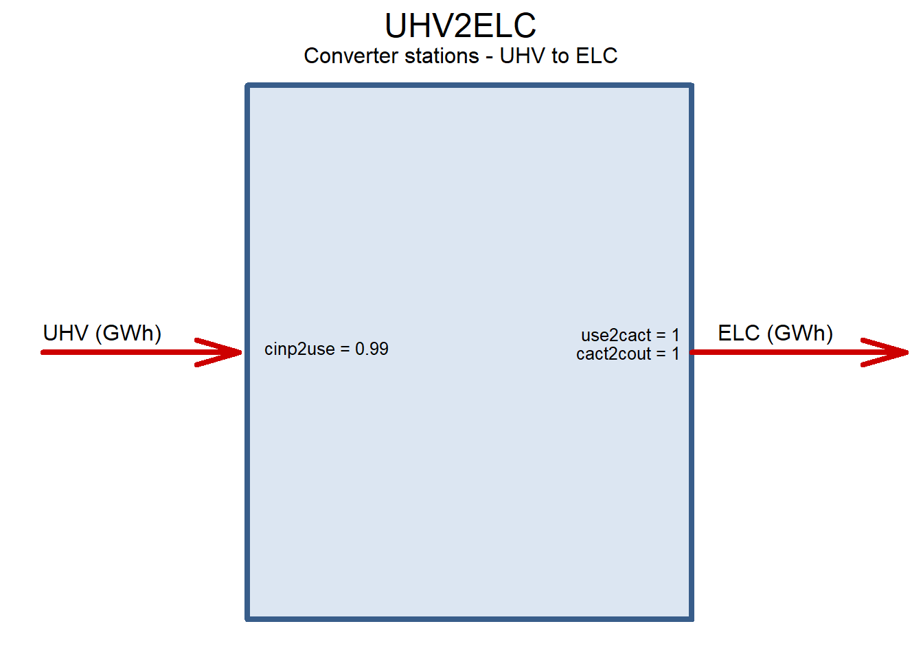
Inverter and rectifier stations
code
# Parameters assumed or calibrated based on
# ABB's 4000-8000 MUSD per 12GW, 2000km, 1-5%
# and other sources

ELC2UHV <- newTechnology(
  name = "ELC2UHV",
  description = "Converter stations - ELC to UHV",
  input = list(
    comm = "ELC",
    unit = "GWh"
    # unit = "PJ"
  ),
  output = list(
    comm = "UHV",
    unit = "GWh"
    # unit = "PJ"
  ),
  # cap2act = 31.536,
  cap2act = 24*365,
  ceff = list(
    comm = "ELC",
    cinp2use = .99 # see also Siemens -- 3% total losses for HVDC/1000km
  ),
  slice = "HOUR",
  invcost = list(
    invcost = 50  #
  ),
  olife = 20 # assumed
)
draw(ELC2UHV)

UHV2ELC <- newTechnology(
  name = "UHV2ELC",
  description = "Converter stations - UHV to ELC",
  input = list(
    comm = "UHV",
    unit = "GWh"
    # unit = "PJ"
  ),
  output = list(
    comm = "ELC",
    unit = "GWh"
    # unit = "PJ"
  ),
  # cap2act = 31.536,
  cap2act = 24*365,
  ceff = list(
    comm = "UHV",
    cinp2use = .99
  ),
  slice = "HOUR",
  invcost = list(
    invcost = 50 # Assumed, based on ABB data
  ),
  olife = 20 # assumed
)
draw(UHV2ELC)
Trade with the rest of the world (ROW)
Currently used to estimate curtailments and the system failure to meet the demand.
code
EEXP <- newExport(
  name = "EEXP",
  description = "Supply curtalments (artificial export to capture excessive ELC production by renewables)",
  commodity = "ELC",
  exp = list(
    price = convert("USD/kWh", "MUSD/GWh", .01/100) # 1/100 cents per kWh
  )
)

EIMP <- newImport(
  name = "EIMP",
  description = "Demand curtailments, electricity import at high price (to identify shortages)",
  commodity = "ELC",
  imp = list(
    price = convert("USD/kWh", "MUSD/GWh", 10) # USD per kWh, marginal price
  )
)

DEMCURT <- newCommodity(
  name = "DEMCURT",
  agg = list(
    comm = "ELC",
    agg = 1
  )
)
# DEMCURT@agg

DIMP <- newImport(
  name = "EIMP",
  description = "Demand curtailments, electricity import at high price (to identify shortages)",
  commodity = "ELC",
  imp = list(
    price = convert("USD/kWh", "MUSD/GWh", 10) # USD per kWh, marginal price
  )
)

# Curtailed demand technology
# i.e. generating technology with high costs
code
# memory managements in GAMS: https://support.gams.com/solver:error_1001_out_of_memory
{gams_options <- "
*$exit
energyRt.holdfixed = 0;
energyRt.dictfile = 0;
option solvelink = 0;
option iterlim = 1e9;
option reslim = 1e7;
option threads = 12;
option LP = CPLEX;
energyRt.OptFile = 1;
*option savepoint = 1;
*option bRatio = 0;
*execute_loadpoint 'energyRt_p';
$onecho > cplex.opt
interactive 1
advind 0
*tuningtilim 2400
aggcutlim 3
aggfill 10
aggind 25
bardisplay 2
parallelmode -1
lpmethod 6
*printoptions 1
names no
freegamsmodel 1
*memoryemphasis 1
threads -1
$offecho
*$exit
"} # GAMS options ####

{cplex_options <- "
interactive 1
CPXPARAM_Advance 0
*tuningtilim 2400
aggcutlim 3
aggfill 10
aggind 25
bardisplay 2
parallelmode -1
lpmethod 6
*printoptions 1
names no
*freegamsmodel 1
*memoryemphasis 1
threads -1
"} # CPLEX parameters ####

{inc4 <-
"parameter zModelStat;
zModelStat = energyRt.ModelStat;
execute_unload 'USENSYS_scenario.gdx';"} # inc4.gms

# if (F) { # Save the workspace (mannual)
# save.image(file = USENSYS$file)
# load(USENSYS$file)
# }

GAMS <- list(
  lang = "GAMS",
  inc3 = gams_options
)

PYOMO <- list(
  lang = "PYOMO",
  files = list(
    cplex.opt = cplex_options
  )
)

JuMP = list(
  lang = "JuMP",
  files = list(
    cplex.opt = cplex_options
  )
)

mobj <- c(mobj, "USENSYS", "GAMS", "PYOMO", "JuMP")

pkgObj <- function(pkg = "energyRt", envir = .GlobalEnv) {
  # returns list of the package objects
  ii <- sapply(ls(envir = envir), function(x) {
    i <- attr(class(get(x, envir = envir)),"package") == pkg
    if(length(i) == 0) i <- F
    i
  })
  names(ii)[ii] # names of objects
}
pkgObj()
##  [1] "BIO"              "CELC2DEM100CAPFX" "CELC2DEM100CAPUP" "CSOL_UP"
##  [5] "CWFF_UP"          "CWIN_UP"          "DEM_ELC_DH"       "DEM_ELC_FX"
##  [9] "DEM100"           "DEM100DEXP"       "DEM35"            "DEM35EXP"
## [13] "DEMCURT"          "DEMY"             "DEMYEXP"          "DIMP"
## [17] "DSMD"             "EBIO"             "EEXP"             "EIMP"
## [21] "ELC"              "ELC2DEM100"       "ELC2DEM35"        "ELC2DEM35CAP"
## [25] "ELC2DSMD"         "ELC2UHV"          "ESOL"             "EWFF"
## [29] "EWIN"             "RES_SOL"          "RES_WFF"          "RES_WIN"
## [33] "route"            "SOL"              "SOLAR_AF"         "STGBTR"
## [37] "STGP2P"           "SUP_BIO"          "TRBD_UHV_NEI"     "TRFX_ELC_NEI"
## [41] "TRFX_UHV_NEI"     "UHV"              "UHV2ELC"          "WFF"
## [45] "WIN"              "WINOF20_AF"       "WINON20_AF"
# save(list = unique(c(pkgObj(), mobj)), file = USENSYS$file)
The Model
The base model and scenario:
- generic electricity (ELC);
- three types of renewables;
- two types of energy storage;
- no inter-regional trade/dispatch.
# Repository with all the data-objects
reps <- add(newRepository('main_repository'),
  # Commodities
  ELC, SOL, WIN, WFF, UHV,
  # Resources (supply)
  RES_SOL, RES_WIN, RES_WFF,
  # Weather factors
  SOLAR_AF, WINOF20_AF, WINON20_AF,
  # Generating technologies
  ESOL, EWIN, EWFF,
  # Storage
  STGBTR
  # STGBTR1,
  # STGP2P1,
  # UHV grid
  # UHV,
  # TRBD_UHV_NEI,
  # ELC2UHV, UHV2ELC
  # Export/Import,
  # EEXP, EIMP,
  # ELC demand with load curve (24 hours x 365 days)
  # DEM_ELC_DH
  # DEM_ELC_FX, # flat
  # Optimized location
  # DEM100,
  # ELC2DEM100,
  # CELC2DEM100CAPFX,
  # CELC2DEM100CAPUP, # optional limit on capacity per region
  # Fixed location, 24h intraday flexibility (DSM)
  # DSMD,
  # ELC2DSMD,
  # >= 35% capacity utilization, optimized location
  # DEM35,
  # ELC2DEM35,
  # DEM35EXP,
  # ELC2DEM35CAP
)
length(reps@data)
names(reps@data)

# model-class object
mdl <- newModel(
  name = 'RENBAL',
  description = "Renewables balancing model",
  ## in case of infeasibility, `dummy` variables can be added
  # debug = data.frame(#comm = "ELC",
  #                    dummyImport = 1e6,
  #                    dummyExport = 1e6),
  region = reg_names,
  discount = 0.05,
  slice = list(ANNUAL = "ANNUAL",
               # MONTH = timeslices$MONTH,
               # HOUR = timeslices$HOUR
               YDAY = timeslices365$YDAY,
               HOUR = timeslices365$HOUR
               ),
  repository = reps,
  GIS = usa49reg,
  early.retirement = F)

# Check the model time-slices
head(mdl@sysInfo@slice@levels)

# Set milestone-years
# mdl <- setMilestoneYears(mdl, start = 2015, interval = c(1, 2, 5, 6, 7, rep(10, 3)))
mdl <- setMilestoneYears(mdl, start = 2018, interval = c(1))
mdl@sysInfo@milestone # check

# (optional) the model info
{mdl@description <- "
USENSYS, power sector, renewables balancing version,
49 regions, 1 hour resolution,
3 types of renewables,
1 types of storages,
Endogenous UHVDC grid,
4 types of demand,
no initial stock."}

# (optional) GAMS and CPLEX options
mdl@misc$includeBeforeSolve <- cplex_options
# (optional) save GDX file with the solution
mdl@misc$includeAfterSolve <- inc_after_solve